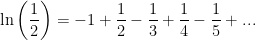
Leibniz’s rule is a powerful tool for solving otherwise impossible integrals. Here is one of these:

Substitution, by parts, partial fractions, try it for yourself, all of these methods will fail to give you an antiderivative. We even had to introduce a special function, named Si(x), just to give it an antiderivative. But our method focuses on solving definite integrals, rather than antiderivatives. “Differentiation under the integral sign”, as we call it, is a direct consequence of Leibniz’s rule, which states
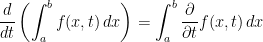
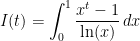
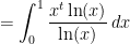
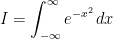
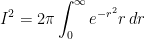
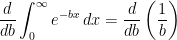
The variable t only serves as a parameter, which hopefully helps us integrate when we take its partial derivative. But this rule basically states that–under certain lenient conditions– one may interchange the derivative operator and the integral. But how does that help us with anything?, you ask. Well here is an example: say you want to calculate this definite integral

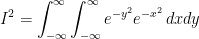
Here again, the usual methods will fail us. And we can’t apply our new rule if we don’t have a parameter t. So let’s introduce a new parameter that, when differentiated, will make it simpler to integrate. Ideally, we would want to get rid of that  in the denominator. What if we set
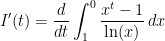
  in the exponent of our integrand? Than our whole expression would be a function of t, let’s call it
  , that we would later evaluate at 2:
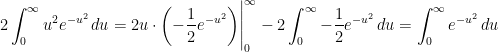
Differentiating with respect to t:
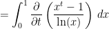

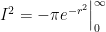
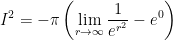
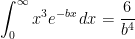
Well this is easier to integrate! The most difficult part is finding the right parameter, and, admittedly, there sometimes won’t be any. But a lot of times, it works nicely just like in our example. We can continue, treating t as a constant in our integration:


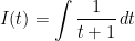
Now, remember, this is the derivative of  , not . But that’s not what we want. So to get our original expression, we need to integrate our result with respect to t:


But what is C? Well let’s see if we can find an “initial” condition from our original integrand.
What happens if we set  ? Then the whole integral equals zero, so
  :
:
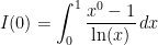
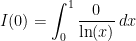

Knowing these conditions, let’s see what our constant is:


Okay, so we don’t have to worry about the constant since it equals zero. So anyways, we want to evaluate our new expression for at , because that’s what we substituted t for in the original integrand. We then get:


And there is our exact result! Interestingly, we had to solve a more general problem, to then apply it specifically to our problem. What we did allows us to generalize:

This technique of integration not only allows us to solve some otherwise resisting integrals, but also to generalize to other parameters! Sometimes, we need to actually add a parameter inside the integrand to be able to evaluate it. This technique was actually popularized by Richard Feynman himself, and this is what he said (well wrote) about it in his book Surely, You’re Joking, Mr. Feynman! :
“I had learned to do integrals by various methods shown in a book that my high school physics teacher Mr. Bader had given me. [It] showed how to differentiate parameters under the integral sign – it’s a certain operation. It turns out that’s not taught very much in the universities; they don’t emphasize it. But I caught on how to use that method, and I used that one damn tool again and again. [If] guys at MIT or Princeton had trouble doing a certain integral, [then] I come along and try differentiating under the integral sign, and often it worked. So I got a great reputation for doing integrals, only because my box of tools was different from everybody else’s, and they had tried all their tools on it before giving the problem to me.”


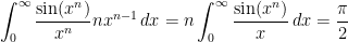

![\displaystyle \int_0^{\infty}\frac{\sin(\sqrt[\pi]{x^3})}{x}\,dx=\zeta(2)=\frac{\pi^2}{6}](https://s0.wp.com/latex.php?latex=%5Cdisplaystyle%C2%A0%5Cint_0%5E%7B%5Cinfty%7D%5Cfrac%7B%5Csin%28%5Csqrt%5B%5Cpi%5D%7Bx%5E3%7D%29%7D%7Bx%7D%5C%2Cdx%3D%5Czeta%282%29%3D%5Cfrac%7B%5Cpi%5E2%7D%7B6%7D&bg=ffffff&fg=000000&s=0&c=20201002)

 . The proof is actually pretty easy, so let’s do it now. It relies on a simple substitution and one iteration of integration by parts.
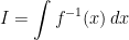
 .
.


 . From our formula,
 , pretty easy:

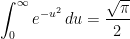
 . We are then looking for
  . After using our dear Pythagoras’ theorem, we end up with the following results:


 -Red Riding Hood and the–hilarious–Big Bag Bolzano-Weierstrass Theorem, this parody is just too good. So yeah, shoutout to the authors for writing this funny story;
  .
.


 et le
et le 
 et
et 


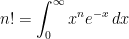
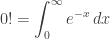
 ? Il doit bien y avoir une façon de calculer ce genre de factorielle non? Eh oui, ça existe, et ça s’appelle la fonction Gamma.
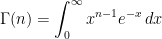


 :
:


 être égal a 1:
 . Par exemple:


 :
:

 revolved around the positive x-axis. This will create a solid of revolution that looks something like this:
 is not defined at that point.


 revolved around the x-axis, we need to use something else: something that factors in the Pythagorean Theorem:

 and
and diverges, then
 will also diverge.
 diverges and we also know that
 Since
Since


 on the interval
  . Since
 will also diverge.