Physics

Posted on September 25, 2017 by philosophicalmath

At what angle should you throw a projectile so that its distance travelled is maximized? You might know that intuitively, that angle should be 45 degrees. Well you’re correct. Now, as an aspiring mathematicians and physicist, I like to prove stuff, and this is no exception. First, we assume that there are no drag forces, and that gravity is the only force acting on our projectile.

So we have an object thrown at an angle $\theta$ thrown with an initial velocity $v$ . Take the origin to be the point of launch, the y-axis the vertical distance above the ground, and the x-axis the horizontal distance from the launch point. We know that the x and y components of the initial velocity are

$\displaystyle v_x=v\cos(\theta)$

$\displaystyle v_y=v\sin(\theta)$

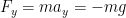
We now have to find the equations of motion for each the x and y components. For this, we’ll use some calculus and Newton’s second law. Let’s first work on the vertical component; we know that the only force acting on our projectile is the force of gravity, pointing in the negative direction. Thus, from Newton, we have

$\displaystyle F_y=ma_y=-mg$

$\displaystyle a_y=-g$

$\displaystyle \frac{d^2y}{dt^2}=-g$

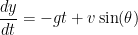
Where the last equation comes form the fact that acceleration is the second derivative of position. We can also express this differential equation like this

$\displaystyle \frac{dv}{dt}=-g$

From here, we can separate and integrate:

$\displaystyle dv=-g\,dt$

$\displaystyle \int\,dv=\int-g\,dt$

$\displaystyle v_y(t)=-gt+v\sin(\theta)$

Our constant was the initial velocity that we derived earlier. We repeat again to solve for position:

$\displaystyle \frac{dy}{dt}=-gt+v\sin(\theta)$

$\displaystyle \int\,dy=\int -gt+v\sin(\theta)\,dt$

$\displaystyle y(t)=-\frac{1}{2}gt^2+v\sin(\theta)t$

And we have no constants because our initial height is zero. Let’s now find the equation of motion in the x direction. Since there are no forces in the x direction, we have zero acceleration, and thus constant velocity.

$\displaystyle v_x(t)=v\cos(\theta)$

$\displaystyle x(t)=v\cos(\theta)t$

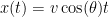
Again, there are no constants because the initial position was the origin. We now have all the information necessary to find the optimal angle of launch. First, we need to find when the projectile hits the ground. This means that

$\displaystyle y(t)=0$

$\displaystyle-\frac{1}{2}gt^2+v\sin(\theta)t=0$

$\displaystyle \left(-\frac{1}{2}gt+v\sin(\theta)\right)t=0$

There are two solutions to this equation. The first one is the initial position of the projectile; we’re not interested in that one. However, the other one is

$\displaystyle t=\frac{2v\sin(\theta)}{g}$

Now, we’re going to substitute this value in our equation of motion for the x direction, since this is what we are trying to maximize.

$\displaystyle x(t)=v\cos(\theta)t$

$\displaystyle x_m=\left(v\cos(\theta)\right)\left(\frac{2v\sin(\theta)}{g}\right)$

$\displaystyle x_m=\frac{2v^2\cos(\theta)\sin(\theta)}{g}$

$\displaystyle x_m=\frac{v^2\sin(2\theta)}{g}$

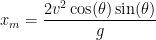
Holding the velocity constant, we are trying to maximize $\sin(2\theta)$ in the interval $\theta\in[0,\frac{\pi}{2}]$ . From trigonometry, this happens when

$\displaystyle \sin(2\theta)=1$

$\displaystyle \theta=\frac{\pi}{4}$

And we know that the value of $\theta$ in degrees is 45. We assumed that the projectile would be launched from an initial height of 0. However, this is not always the case. In a future post, we’ll look at the more general case.

Convergence of functional sequences

Posted on September 13, 2017 by philosophicalmath

What does it mean for a sequence to converge? What does it mean for a sum to converge? Are there different types of convergence? All these question are fundamental to mathematics, and are usually covered in a Real Analysis class. Even though I–unfortunately–haven’t yet taken that course, I am fascinated by the different mathematical concepts it covers. One of these is the idea of convergence. We’ll focus on the two main types: pointwise convergence and uniform convergence.

Since pointwise convergence is “weaker”, in a sense, than uniform convergence, I think it’s natural to start with it. Here is the formal definition:

Let a sequence of functions $(f_n)_{n=1}^{\infty}$ be defined on an interval $I\subseteq\mathbb{R}$ where $f_n: I\to\mathbb{R} \,\,\,\,\forall n\in\mathbb{N}$ . The sequence converges pointwise to a function $f:I\to\mathbb{R}$ if

$\displaystyle \lim_{n\to\infty} f_n(x)=f(x)$

For example, consider the sequence

$\displaystyle f_n(x)=x-\frac{1}{n}$

It is easy to verify that our sequence converges pointwise to the limit function $f(x)=x$ . Indeed,

$\displaystyle \lim_{n\to\infty} \left(x-\frac{1}{n}\right)=x$

Now for a little harder example; let the following define a sequence of functions:

$\displaystyle f_n(x)=e^{-nx}$ for $x\in[1,5]$

Does our sequence converge pointwise on that interval? Let’s check:

$\displaystyle \lim_{n\to\infty} e^{-nx}=0 \,\,\,\forall x\in[1,5]$

Thus our sequence converges to the limit function $f(x)=0$ on the interval $[1,5]$ . But what happens if we look at the interval $[0,5]$ ? We know that

$\displaystyle e^{-nx}\to 0 \,\,\,\forall x\in(0,5]$ pointwise.

However $f_n(0)=1$ for all $n$ . This means the limit function is not continuous, despite the fact that every $f_n(x)$ is continuous.

This points to one of the flaws of pointwise convergence: it does not guarantee continuity, and nor does it guarantee differentiability. We need a stronger form of convergence: uniform convergence. But first, there is one definition that we need. Define the supremum norm of $f$ on $I$ as

$\displaystyle||f||_I=\sup_{x\in I}|f(x)|$

We are now ready:

$\displaystyle ||f_n(x)-f(x)||_I\to 0 \,\,\,\,\,\text{as} \,\,\,\, n\to\infty$

Notice that uniform convergence implies pointwise convergence. We can now look at a previous sequence of functions that we know to be pointwise convergent, and check whether it is uniformly convergent. We know that the sequence $f_n(x)=e^{-nx}$ converges pointwise on $[1,5]$ . Checking for uniform convergence:

$\displaystyle ||e^{-nx}-0||_{x\in[1,5]}=||e^{-nx}||_{x\in[1,5]}$

$\displaystyle =e^{-n}\to 0 \,\,\,\,\text{as}\,\,\,\, n\to\infty$

Thus the sequence converges uniformly on the interval $[1,5]$ . Let’s now look at a different sequence:

$\displaystyle f_n(x)=xe^{-nx}\,\,\,\text{on}\,\,\,[0,\infty)$

It is easily verified that the sequence converges pointwise to the limit function $f(x)=0$ . What about uniform convergence?

$\displaystyle ||xe^{-nx}||_{x\in[0,\infty)}=\sup_{x\in[0,\infty)}|xe^{-nx}|$

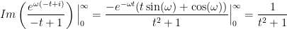
After differentiating $f_n(x)$ we have that the function attains a maximum at $x=\frac{1}{n}$ .

$\displaystyle \sup_{x\in[0,\infty)}|xe^{-nx}|=f_n\left(\frac{1}{n}\right)$

$\displaystyle =\frac{1}{ne}\to 0\,\,\,\text{as}\,\,\, n\to\infty$

Thus our sequence converges uniformly to its limit function $f(x)=0$ on $[0,\infty)$ .

There are many applications of uniform convergence, including the guarantee that the limit function is continuous and differentiable if the sequence function is. These types of convergence can be extended to functional series, with some very interesting results.

Alternating harmonic series

Posted on September 12, 2017 by philosophicalmath

It’s a classic result that $\zeta(1)$ , the harmonic series, diverges. But what about the alternating version of the series? And if it converges, what is its sum? Here is the series:

$\displaystyle \sum_{n=1}^{\infty} \frac{(-1)^{n-1}}{n}=1-\frac{1}{2}+\frac{1}{3}-\frac{1}{4}+\frac{1}{5}-...$

We can first use the alternating series test for convergence. We need the limit to be 0:

$\displaystyle \lim_{n\to\infty}\left(\frac{(-1)^{n-1}}{n}\right)=0$

Now, all we have to is to prove that it is our terms are decreasing. Mathematically,

$\displaystyle a_n=\frac{(-1)^{n-1}}{n}$

$\displaystyle |a_n|>|a_{n+1}|$

And this is true for our series because

$\displaystyle \frac{1}{n}>\frac{1}{n+1}$

So we now know that our series converges. Let’s try to find its sum. We can use the fact that

$\displaystyle \frac{1}{1+x}=\sum_{n=0}^{\infty} (-1)^n x^n\,\,\,\,\,\forall|x|<1$

Integrating both sides:

$\displaystyle \int \frac{1}{1+x}\,dx=\int\sum_{n=0}^{\infty} (-1)^n x^n\,dx$

Fubini’s theorem lets us switch integral and sum; we then have

$\displaystyle \ln(1+x)=\sum_{n=0}^{\infty} (-1)^n \frac{x^{n+1}}{n+1}$

Or, changing the index of summation,

$\displaystyle \ln(1+x)=\sum_{n=1}^{\infty} (-1)^{n-1} \frac{x^{n}}{n}$

And notice that for $x=1$ , we have the alternating harmonic series:

$\displaystyle \ln(1+1)=\sum_{n=1}^{\infty} \frac{(-1)^{n-1}}{n}$

$\displaystyle \ln(2)=\sum_{n=1}^{\infty} \frac{(-1)^{n-1}}{n}$

$\displaystyle \ln(2)=1-\frac{1}{2}+\frac{1}{3}-\frac{1}{4}+\frac{1}{5}-...$

And there is our sum! If you are worried about convergence issues because 1 is at the endpoint of the interval of convergence, remember that we already proved the the series converges.

We can also get another interesting result:

$\displaystyle \ln(2)=\sum_{n=1}^{\infty} \frac{(-1)^{n-1}}{n}$

$\displaystyle \ln(2)=-\sum_{n=1}^{\infty} \frac{(-1)^{n}}{n}$

$\displaystyle \ln\left(\frac{1}{2}\right)=\sum_{n=1}^{\infty} \frac{(-1)^{n}}{n}$

$\displaystyle \ln\left(\frac{1}{2}\right)=-1+\frac{1}{2}-\frac{1}{3}+\frac{1}{4}-\frac{1}{5}+...$

A Dirichlet integral

Posted on September 4, 2017 by philosophicalmath

Let’s look at one of the most famous definite integrals,

$\displaystyle \int_0^{\infty} \frac{\sin(\omega)}{\omega}\,d\omega$

This integral is particularly interesting because it doesn’t yield itself to the standard techniques of integration. What makes it even more interesting are the multitude of ways of evaluating it. Laplace transforms, double integrals and differentiation under the integral sign all work here. I’ll choose to focus on the double integral method; if you wish to learn more about evaluating it using differentiation under the integral sign, you should watch this video, from a friend of mine who does a phenomenal job at explaining it.

Mathematics is not an exact science, like some people tend to think. Especially when talking about integrals. I like to view them as an art, where one needs ample creativity to be proficient in it. And because of this, sometimes there appears to be no logic going from one step to another. This the case here.

To start, first notice that

$\displaystyle \frac{\sin(\omega)}{\omega}=\int_0^{\infty} e^{-\omega t}\sin(\omega)\,dt$

This is what I’m talking about. There is no formula that will lead you to use this fact. Instead, the first person who used this technique was creative enough to come up with this and use it in the evaluation of the integral.

Let’s make a substitution in our original integrand:

$\displaystyle \int_0^{\infty} \frac{\sin(\omega)}{\omega}\,d\omega= \int_0^{\infty}\left(\int_0^{\infty} e^{-\omega t}\sin(\omega)\,dt\right) \,d\omega=\int_0^{\infty}\int_0^{\infty} e^{-\omega t}\sin(\omega)\,dt d\omega$

We now have a double integral to evaluate. And while you may think this only further complicated the task, it actually helped us. We can now change the order of integration*, a classic move in the evaluation of double integrals.

$\displaystyle \int_0^{\infty}\int_0^{\infty} e^{-\omega t}\sin(\omega)\,dt d\omega=\int_0^{\infty}\int_0^{\infty} e^{-\omega t}\sin(\omega)\,d\omega dt$

The inner integral can be solved easily by integration by parts, but I prefer a different approach. Note that

$\displaystyle Im(e^{i\omega})=\sin(\omega)$

Focusing on the inner integral, we can equate these:

$\displaystyle \int_0^{\infty} e^{-\omega t}\sin(\omega)\,d\omega=Im\int_0^{\infty} e^{-\omega t}e^{i\omega}\,d\omega=Im\int_0^{\infty} e^{\omega(-t+i)}\,d\omega=\left(Im\frac{e^{\omega(-t+i)}}{-t+i}\right)\Big|_0^{\infty}$

To be able to evaluate this, we need to find its imaginary part. After using conjugates and doing some simple arithmetic, we arrive at the result:

$\displaystyle Im\left(\frac{e^{\omega(-t+i)}}{-t+1}\right)\Big|_0^{\infty}=\frac{-e^{-\omega t}(t\sin(\omega)+\cos(\omega))}{t^2+1}\Big|_0^{\infty}=\frac{1}{t^2+1}$

Remember that this was the inner integral. So we can substitute our new expression back in our original double integral:

$\displaystyle \int_0^{\infty}\int_0^{\infty} e^{-\omega t}\sin(\omega)\,d\omega dt=\int_0^{\infty} \frac{1}{t^2+1}\,dt$

$\displaystyle =\lim_{b\to\infty}\left(\arctan(t)\Big|_0^{b}\right)=\lim_{b\to\infty}\arctan(b)=\boxed{\frac{\pi}{2}}$

Thus,

$\displaystyle \int_0^{\infty} \frac{\sin(\omega)}{\omega}\,d\omega=\frac{\pi}{2}$

Since our function is even, the integral over the whole real line gives

$\displaystyle \int_{-\infty}^{\infty} \frac{\sin(\omega)}{\omega}\,d\omega=2\left(\frac{\pi}{2}\right)=\pi$

And there’s more! After solving an integral like that, you can make a substitution to get a new result. In this case, if we let

$\displaystyle \omega=x^3$

$\displaystyle d\omega=3x^2\,dx$

$\displaystyle \int_0^{\infty} \frac{\sin(\omega)}{\omega}\,d\omega=3\int_0^{\infty} \frac{\sin(x^3)}{x}\,dx=\frac{\pi}{2}$

This means that

$\displaystyle \int_0^{\infty} \frac{\sin(x^3)}{x}\,dx=\frac{\pi}{6}$

Doubling the interval of integration,

$\displaystyle \int_{-\infty}^{\infty} \frac{\sin(x^3)}{x}\,dx=\frac{\pi}{3}$

I think that’s so cool!

We can even generalize for other powers of x. Make the substitution

$\displaystyle \omega=x^n$

$\displaystyle d\omega=nx^{n-1}\,dx$

$\displaystyle \int_0^{\infty} \frac{\sin(x^n)}{x^n} nx^{n-1}\,dx=n\int_0^{\infty}\frac{\sin(x^n)}{x}\,dx=\frac{\pi}{2}$

$\displaystyle\int_0^{\infty}\frac{\sin(x^n)}{x}\,dx=\frac{\pi}{2n}$

Finally, with this, we can now construct a rather exotic, but beautiful, equality:

$\displaystyle \int_0^{\infty}\frac{\sin(\sqrt[\pi]{x^3})}{x}\,dx=\zeta(2)=\frac{\pi^2}{6}$

*For a rigorous proof that changing the order of integration is possible, see here.

Mathematical Poetry

Mathematical musings and updates

Monthly Archives: September 2017

Physics

Convergence of functional sequences

Alternating harmonic series

A Dirichlet integral