A surprising integral

Today, we are interested in the following integral:

\begin{aligned}  I\equiv\int_0^\infty \frac{x\log(x)}{(1+x^2)^2}\,dx.\end{aligned}

I found this integral timidly hiding in a question on Math.StackExchange, where there were already several answers, much shorter than mine. But, as you will see, I think there is something valuable in my longer approach.

The first idea I thought of when seeing that logarithm in the numerator is differentiation under the integral sign. And that’s exactly what we’ll use. As usual in these cases, we consider a parameterization of the type

\begin{aligned}  I(\alpha)\equiv\int_0^\infty \frac{x^\alpha}{(1+x^2)^2}\,dx.\end{aligned}

We immediately see that our desired integral is I=I'(1). Our goal is then simply to compute I(\alpha), differentiate with respect to \alpha, and let \alpha \to 1. However, there will be a few surprises along the way. Let’s get started.

Our first step is to substitute x^2=k, and note that our interval [0,\infty) is simply mapped to itself after this change of variables. We find that

\begin{aligned}  I(\alpha)=\frac{1}{2}\int_0^\infty \frac{k^{\alpha/2}}{(1+k)^2}\,\frac{dk}{\sqrt{k}}.\end{aligned}

At this point, we see that our integral can be expressed in terms of the Beta function, B(m,n), which itself can be expanded into an expression involving Gamma functions:

\begin{aligned}  \frac{1}{2}\int_0^\infty \frac{k^{\alpha/2}}{(1+k)^2}\,\frac{dk}{\sqrt{k}}&=\frac{1}{2}B(\alpha/2+1/2, 3/2-\alpha/2) \\ &=\frac{1}{2}\frac{\Gamma(\alpha/2+1/2)\Gamma(3/2-\alpha/2)}{\Gamma(\alpha/2+1/2+3/2-\alpha/2)} \\ &= \frac{1}{2}\Gamma(\alpha/2+1/2)\Gamma(3/2-\alpha/2).\end{aligned}

We are excruciatingly close to being able to apply the reflection formula for the Gamma function,

\begin{aligned}  \Gamma(z)\Gamma(1-z)=\frac{\pi}{\sin(\pi z)},\end{aligned}

but are unable to. To remedy this situation, we can use the recursive property of the Gamma function, z\Gamma(z)=\Gamma(z+1), or in a form more useful to us,

\begin{aligned}  \Gamma(z)=(z-1)\Gamma(z-1).\end{aligned}

Applying this identity to the second Gamma function in our expression for I(\alpha), we can now use the reflection formula:

\begin{aligned}  \frac{1}{2}\Gamma(\alpha/2+1/2)\Gamma(3/2-\alpha/2) &= \frac{1}{2}\Gamma(\alpha/2+1/2)\Gamma(1/2-\alpha/2)\left(\frac{1-\alpha}{2}\right) \\ &= \left(\frac{1-\alpha}{4}\right) \Gamma(1/2+\alpha/2)\Gamma(1-(1/2+\alpha/2)) \\ &= \left(\frac{1-\alpha}{4}\right) \frac{\pi}{\sin(\pi\alpha/2+\pi/2)} \\ &= \left(\frac{1-\alpha}{4}\right) \frac{\pi}{\cos(\pi\alpha/2)}.\end{aligned}

Differentiating with respect to \alpha, we obtain

\begin{aligned}  I'(\alpha)=\frac{\pi}{4}\left[ \frac{(1-\alpha)\sin(\pi\alpha/2)\pi/2-\cos(\pi\alpha/2)}{\cos^2(\pi\alpha/2)}\right]\end{aligned}

To take the \alpha \to 1 limit, we apply l’Hopital’s rule to arrive at the following

\begin{aligned} \lim_{\alpha\to 1}I'(\alpha) &= -\frac{\pi}{8} \lim_{\alpha\to 1}\frac{(1-\alpha)\cos(\alpha\pi/2)}{\cos(\alpha\pi/2)\sin(\alpha\pi/2)}=0 \end{aligned}

And, somewhat unexpectedly, we find (well, ignoring some subtleties associated with the interchange of the limit and integral, which can be taken care of with a suitable application of the dominated convergence theorem),

\begin{aligned} \boxed{\int_0^\infty \frac{x\log(x)}{(1+x^2)^2}\,dx=0}\end{aligned}

Indeed, the negative signed area on the interval [0,1] has perfectly canceled the positive signed area on [1,\infty). This seems rather improbable and surprising—but is elegant.

I told you at the beginning of the post that this approach to this integral has some advantages over other, shorter ones. And indeed, it can be applied to much more general integrals, which I’ll explore in a future post, that are of the form

\begin{aligned} \int_0^\infty \frac{x^\alpha \log^m(x)}{(\beta^\gamma+x^\chi)^\mu}\,dx,\end{aligned}

where \text{Re}\,\alpha>-1, \text{Re}\,\chi, \text{Re}\,\mu>0, \text{Re}\,(\chi\mu-\alpha)>1, m\in\mathbb{N}, and \beta, \gamma\in\mathbb{C}. Thanks for reading!

Hamilton’s principle, Euler-Lagrange’s equations and a simple symmetry consideration

Hello everyone, today we we will be looking at a set of fundamental equations in physics: the Euler-Lagrange equations. These mathematical relations govern the evolution of classical systems, whether that be simple projectile motion or electromagnetic fields, and also intervene in quantum theories. They originate from Hamilton’s principle, which states that there is a certain quantity, named the Action, that is always stationary for every possible time evolution of a system’s configuration’s space. We will discuss the Euler-Lagrange equations and their derivations while ignoring some of the mathematical formalities i.e. it will be a physicist’s derivation.

First, define the action \mathcal{S} as

\begin{aligned}  \mathcal{S}=\int_{t_1}^{t_2} L(q^i(t),\dot{q}^i(t), t)\,dt  \end{aligned}

Where L is the Lagrangian, and is defined as the difference of kinetic and potential energy: L=T-U, q^i(t) are the different coordinates required to determine the state of the system, and \dot{} denotes differentiation with respect to time. Hamilton’s principle states that a classical system will follow a path which makes, the Action stationary, more specifically to first order:

\begin{aligned}  \delta\mathcal{S}=0 \end{aligned}

Where \delta \mathcal{S}=S(q+\delta q) - S(q) where \delta q(t) is a small perturbation that is zero at the endpoint of the path: \delta(q(t_1))=\delta(q(t_2))=0. Using Taylor expansions on the first term we see that

\begin{aligned}  \int_{t_1}^{t_2}\frac{\partial L}{\partial q^i}\delta q^i+\frac{\partial L}{\partial \dot{q}^i}\delta \dot{q}^i\,dt=0 \end{aligned}

Integrating the second term in the integrand by parts, and using the fact that our variations vanish on the boundaries, we find that

\begin{aligned}  \int_{t_1}^{t_2}\delta q^i\left(\frac{\partial L}{\partial q^i}-\frac{d}{dt}\frac{\partial L}{\partial \dot{q}^i}\right)\,dt=0 \end{aligned}

Appealing to the Fundamental Lemma Calculus of Variations, it must be that

\begin{aligned}  \frac{\partial L}{\partial q^i}-\frac{d}{dt}\frac{\partial L}{\partial \dot{q}^i}=0 \end{aligned}

for each degree of freedom q^i(t). Applying what we have just derived to a particle in one dimension subject to a potential U(x), and with kinetic energy \frac{1}{2} m\dot{x}^2, its equation of motion is given by

\begin{aligned}  m\ddot{x}=-\frac{\partial U}{\partial x} \end{aligned}

which is exactly Newton’s law, where the force is given by -\nabla{U}, in the case of one dimension.

It is now interesting to turn to the study of transformations on the Lagrangian and observe their effects on the Euler-Lagrange equations, or equations of motion. First, notice that multiplying the Lagrangian, or Action, by a constant does not change the path that the system will take.

I owe this elegant observation to the textbook “Mechanics“, from the series “Course in Theoretical Physics“, by the Russian physicists Landau and Lifshitz. Assume that the potential is a homogenous function of the coordinates q^i, meaning that there exists some m such that U(\alpha q^i)=\alpha^m U(q^i). The common potentials, such as U(r)\propto 1/r, U(x)\propto x^2, and U(h)\propto h, which are the general gravitational potential, the oscillator potential, and the gravitational potential near the earth respectively, where g can be treated as constant, are all homogenous with, respectively, m=-1, m=2, m=1. Now, if we make a transformation and shift the time by a factor \beta and the positions by a factor of, say, \alpha: {q^i}'=\alpha q^i. The potential, being homogenous, will then be simplify multiplied by a factor: U(\alpha q^i)=\alpha^m U(q^i). The kinetic energy will then change by a factor of \alpha^2/\beta^2. If we set these equal to each other, and find that then it must be that \beta=\alpha^{1-m/2}, the Lagrangian is multiplied by a constant, and thus the fundamental equations of motion remain the same. These Lagrangian different by this constant are geometrically similar path, but differ in just size, as Landau and Lifshitz put it. By constructing these various path, which all have to obey the same equations of motion if \beta=\alpha^{1-m/2} is satisfied, then we can derive various useful and interesting relationship between dynamical variables. I will first show how to investigate the connection between changes in time, and in position, or length l.

First, we look at the ratio t'/t=\beta. Next, at the ratio l'/l=\alpha. Our constraint is that, for these times and positions to be part of the same paths, (geometrically) it must be that \beta=\alpha^{1-m/2}. Thus we find that

t'/t=\left(l'/l\right)^{1-m/2}

Another way of saying this is

t\propto l^{1-m/2}

Thus,

l\propto t^{2/(2-m)}

This is a very powerful and general relationship that we just derived from symmetry considerations. As an example of its usefulness, let’s look at the classic gravitational potential where m=-1:

t\propto l^{3/2}

Which is Kepler’s third law for the period t and the semi-major axis l .

For the oscillatory potential, where m=2, we find that

t\propto l^0=1

Meaning that the period t is independent of the amplitude of the motion l . Seem familiar?

Take m=1 to investigate the near-earth-gravitational potential U=mgh to see that

l\propto t^2

Which agrees with the kinematical formula h=\frac{1}{2}gt^2.

We are not just restricted to time and position though. Indeed, the general procedure is to express the relevant quantities, whose proportionality we want to investigate, in terms of \alpha=t'/t and \beta=q'/q before applying the constraint \beta=\alpha^{1-m/2}. Granted, this technique will only work with homogeneous potentials.

For example, say we are interested in seeing how the velocity v varies with position l. Then, we are trying to find the constant \gamma such that

v'/v=(l'/l)^\gamma

Since v'/v=\alpha/\beta and l'/l=\beta,

\alpha/\beta=\alpha^\gamma

Or

\beta=\alpha^{1-\gamma}

Because of our constraint, this implies that 1-\gamma=1-m/2, or \gamma=m/2. Thus

v\propto l^{m/2}

For the near-earth gravitational potential, we have v\propto \sqrt{l}, agreeing with the familiar v=\sqrt{2gh}. For the more general case of classical gravity, this result gives v\propto  1/\sqrt{l}, which we can also derive by application of the principles of circular motion.

I thought I’d share this method of deriving various useful relationships for homogeneous potentials as I have never seen it outside of Landau and Lifshitz’s text. Not to mention that symmetry considerations are ubiquitous in many different areas of physics.

Cauchy and finite-interval integrals

This time, we’ll be looking at a technique from complex analysis to solve a class of trigonometric integrals on the unit circle, or [0,2\pi]. We’ll begin by studying this integral:

\begin{aligned} \int_0^{2\pi} \frac{1}{(1-a\cos \theta)^2} \,d\theta \end{aligned}.

For this integral to even converge, we have to have |a| less than one, as that guarantees that there won’t be any singularity (which wouldn’t be integrable) of the function. At first, view this integral seems pretty hard to compute if we rely on just real analytic approaches. Which is why we’ll be switching over to working with complex numbers, where we can use Cauchy’s integral formula:

\begin{aligned}  \int_\gamma \frac{f(z)}{z-\omega} \,dz=2\pi i f(\omega) \end{aligned},

where \gamma is a circle of a radius r, f is holomorphic on the disk of the same radius, and |\omega|<r.

Going back to our original integral and using the complex exponential form of cosine, our integral is now

\begin{aligned}  \int_0^{2\pi} \frac{dz}{\big(1-ae^{i\theta}/2-ae^{-i\theta}/2\big)^2} \end{aligned}.

After substituting e^{i\theta}=z, dz/iz=d\theta, our integral transforms into

\begin{aligned}  &=\int_\gamma \frac{dz}{iz} \frac{1}{\big(1-az/2-a/2z \big)^2} \\ &= -\frac{4i}{a^2} \int_\gamma  \frac{z}{\big(z^2-2z/a-1 \big)^2}\,dz\end{aligned}

Where \gamma is the unit circle on the Argand diagram. Now, to be able to apply Cauchy’s theorem, we have to factor the denominator into the form (z-s)(z-\sigma), where one of s or \sigma is included in our unit circle. We can do this pretty quickly using the quadratic formula:

\begin{aligned}  s&=\frac{1-\sqrt{1-a^2}}{a} \\ \sigma &= \frac{1+\sqrt{1-a^2}}{a}\end{aligned}.

First, we can notice that because |a| is less than one, our roots will always be real, as the discriminant inside the square root will always be positive. Because a is relatively small, we can approximate both of these roots using the first two terms of the binomial series:

\begin{aligned}  s&\approx a/2 \\ \sigma &\approx \frac{2}{a} - \frac{a}{2} \end{aligned}.

We can see that for a\in(-1,1), s will always be in the unit circle while \sigma will alway be outside of our circle. Going back to our original integral and factoring the denominator, it can be expressed in this form:

\begin{aligned}  -\frac{4i}{a^2} \int_\gamma  \frac{z/(z-\sigma)^2}{(z-s)^2}\,dz\end{aligned}

We are close to being able to apply Cauchy’s formula, but not quite there, as our denominator in our integrals is raised to the second power. To fix this, differentiate both sides of Cauchy’s formula with respect to \omega to obtain

\begin{aligned}  \int_\gamma \frac{f(z)}{(z-\omega)^2} \,dz=2\pi i f^{(1)}(\omega) \end{aligned}.

Applying it to our case by letting f(z)=-4iz/a^2(z-\sigma)^2, our integral reduces to

\begin{aligned}  -\frac{4i}{a^2} \int_\gamma  \frac{z/(z-\sigma)^2}{(z-s)^2}\,dz=-2\pi i \frac{d}{dz}\frac{4iz}{a^2(z-\sigma)^2} \Biggr|_{z=s}\end{aligned}

Carrying out the computations,

\begin{aligned}  -\frac{4i}{a^2} \int_\gamma  \frac{z/(z-\sigma)^2}{(z-s)^2}\,dz=\frac{2\pi}{(1-a^2)^{3/2}} \end{aligned}.

We have then also found the value of our original integral:

\begin{aligned} \int_0^{2\pi} \frac{1}{(1-a\cos \theta)^2} \,d\theta = \frac{2\pi}{(1-a^2)^{3/2}}\end{aligned}.

I’d still like to show at least one of the ways through which real techniques can be used to calculate this integral. First, we’ll look at the following integral, where |a|<|b|:

\begin{aligned} I(a,b)=\int_0^{2\pi} \frac{1}{b-a\cos \theta} \,d\theta =  \frac{1}{b} \int_0^{2\pi} \frac{1}{1-(a/b)\cos \theta} \,d\theta\end{aligned}.

Notice that

\begin{aligned} \partial_b I(a,b)\Big|_{b=1}=-\int_0^{2\pi} \frac{1}{(1-a\cos \theta)^2} \,d\theta\end{aligned}.

Which is our original integral. Because |(a/b)\cos\theta|\le|a/b|<1, we can expand the integrand into its geometric series and switch summation and integration, obtaining

\begin{aligned} \frac{1}{b}\sum_{n\ge 0} \Big(\frac{a}{b}\Big)^n \int_0^{2\pi} \cos^n\theta \,d\theta \end{aligned}.

Usually I would jump to the Beta function to evaluate the last integral, but today I decided to use a different approach that I don’t think has appeared on the blog yet. First, we can see that from the complex exponential definition of the cosine function and the binomial theorem,

\begin{aligned} \cos^n \theta=2^{-n} \sum_{k=0}^n {n \choose k} e^{i\theta(2k-n)} \end{aligned}.

Now, owing to the orthogonality of the complex exponential, we have that

\begin{aligned}  \int_0^{2\pi} \cos^n \theta \,d\theta = 2\pi 2^{-n}\sum_{k=0}^n {n \choose k} \delta(2k,n)\end{aligned}

Where \delta is the Kronecker Delta. It will pick out the term of the sum in which k=n/2, which is only possible if n is even, meaning that m=n/2 for some integer m. If n is odd, the sum is zero, letting us substitute in the relevant n=2m:

\begin{aligned}  \int_0^{2\pi} \cos^{2m} \theta \,d\theta = 2\pi 2^{-2m}\sum_{k=0}^{2m} {2m \choose k} \delta(2k,2m)\end{aligned}

The only term left in the sum, thanks to the Kronecker Delta, is the term k=m:

\begin{aligned}  \int_0^{2\pi} \cos^{2m} \theta \,d\theta = 2\pi 2^{-2m} {2m \choose m} \end{aligned}

Going back to our infinite sum, we find that the only non-vanishing terms will occur, as we said, when n is even, or in other words when n=2m. Our series is now

\begin{aligned} \frac{2\pi}{b}\sum_{m\ge 0} 2^{-2m}\Big(\frac{a}{b}\Big)^{2m}  {2m \choose m} \end{aligned}.

This form is actually closely related to a series representation of the arcsine function:

\begin{aligned} \arcsin x=\sum_{m\ge 0} 2^{-2m}  {2m \choose m} \frac{x^{2m+1}}{2m+1} \end{aligned}.

Notice that if we can interchange the derivative and summation operator (actually the limit of the finite sum), our series reduces to

\begin{aligned} &=\frac{2\pi}{b} \arcsin' \left(\frac{a}{b}\right) \\ &= \frac{2\pi}{b}\frac{1}{\sqrt{1-(a/b)^2}} \\ &= \frac{2\pi}{\sqrt{b^2-a^2}} \end{aligned}.

Now, in order to justify this switch of limit operators, we can use the Weierstrass M-test, which states that if f_n(x):X\to I is a sequence of functions, and there exists a sequence M_n such that |f_n(x)|\le M_n for every n\in\mathbb{N} and all x\in X and \sum_{n\ge 0}  M_n converges, then \sum_{n\ge 0}  f_n(x) converges uniformly. Why is it useful to know that a series of functions converges uniformly? Well, if the sum g(x)=\sum_{n\ge 0} g_n(x):X\to I converges at a least one point x\in X, and \sum_{n\ge 0} g'_n(x) converges uniformly, then g'(x)=\frac{d}{dx} \sum_{n\ge 0} g_n(x)=\sum_{n\ge 0} \frac{d}{dx} g_n(x).

All this means that if we can prove that the series \sum_{m\ge 0} {2m \choose m} 2^{-2m}x^{2m} converges uniformly, then we can indeed differentiate term by term the series for arcsine and obtain our result.

Letting a_m= {2m \choose m} 2^{-2m}, we first see that |a_m x^{2m}|\le |a_m x^{m}| on our interval of interest. Let x_\epsilon=1-\epsilon for \epsilon\in(0,2). I will show that our series converges uniformly for any x<x_\epsilon, meaning for any x\in(-1,1) because we can make \epsilon as small as we want. We have to see that our sequence a_m x^{m} is bounded by a constant, since its series converges, say by M. Notice that |a_m x^m|=|a_m x^m|\le |a_m x^m| |x^m_\epsilon| < M |x^m_\epsilon|. The series of this last sequence converges, as it is geometric and x_\epsilon=1-\epsilon<1. Thus, \Big|{2m \choose m} 2^{-2m} x^{2m}\Big |< M |x^m_\epsilon|, and because the series of the latter sequence converges, by the M-test the series \sum_{m\ge 0}{2m \choose m} 2^{-2m} x^{2m} converges uniformly. Thanks to this result and the fact that the series for arcsine term does converge for at least one x\in(-1,1), we can indeed differentiate the series term by term.

This justifies all of our results, and thus

\begin{aligned} \int_0^{2\pi} \frac{1}{b-a\cos\theta}\,d\theta= \frac{2\pi}{\sqrt{b^2-a^2}}\end{aligned}.

Differentiating both sides and setting b=1, we obtain again the same result:

\begin{aligned} \int_0^{2\pi} \frac{1}{(1-a\cos \theta)^2} \,d\theta = \frac{2\pi}{(1-a^2)^{3/2}}\end{aligned}.

Although it took us a bit longer to arrive at the result by real analytic techniques, we also encountered some interesting mathematics along the way. Thanks for reading!

Ramanujan & Feynman

Hello! Today, we’ll be exploring a certain integral that will allow us to use a combination of Ramanujan’s Master Theorem and Feynman’s technique to evaluate it. This integral was actually one of the first ones in which I used an extension (if you can call it that) of the master theorem to compute integrals that don’t exactly satisfy the necessary conditions at first sight.

Anyway, here’s this posts’s integral

\begin{aligned} \int_0^\infty\sin (x^2) \log^2 x\,dx  \end{aligned}

You might first doubt that the integrand f is even integrable—after all, it doesn’t even vanish as x\to\infty. Here is a plot of it:

As you can see, the function rapidly oscillates as its input grows. So fast, even, that it’s Riemann integral on [0,\infty) remains finite. It is, however, not Lebesgue integrable as it depends on the oscillations of the sine function. In order to better see this, substitute \sqrt{u}=x. Our integral then becomes

\begin{aligned} I=\frac{1}{8} \int_0^\infty \frac{\sin (u)}{\sqrt{u}} \log^2 u\,du \end{aligned}

It is easier to see how this integral converges with this representation. Now in order to actually evaluate it, we can notice that it is just the second derivative evaluated at zero of another integral:

\begin{aligned} I=\frac{d^2}{da^2} \Big|_{a=0} \int_0^\infty x^a  \sin(x^2) \,dx \end{aligned}

We are basically taking a Mellin transform and evaluating it so that the polynomial factor term is unity. Here is where Ramanujan’s Master Theorem will be helpful. As a reminder, this theorem states that if a function g can be expanded in a Taylor series around zero as such:

\begin{aligned} g(x)=\sum_{k\ge 0} \frac{(-x)^k}{k!} \phi(k)\end{aligned}

Then its Mellin transform is given by

\begin{aligned} \int_0^\infty x^{s-1} g(x)=\Gamma(s) \phi(-s) \end{aligned}

In our case, we can expand our function as

\begin{aligned} \sin(x^2)=\sum_{k\ge 0} \frac{(-1)^k x^{4k+2}}{k!} \frac{k!}{(2k+1)!}\end{aligned}

We can see that the problem is the power of x. However, if we let \sqrt[4]{\omega}=x and move some factors around, we find that

\begin{aligned} \frac{\sin(\sqrt{\omega})}{\sqrt{\omega}} =\sum_{k\ge 0} \frac{(-x)^k}{k!} \frac{k!}{(2k+1)!}\end{aligned}

And this function does indeed satisfy the conditions needed for the master theorem, with \phi(k)=k!/(2k+1)!. As will soon become clear why, we will let b=a/4 in our previous integral. We are thus looking for

\begin{aligned} I=\frac{1}{16}\frac{d^2}{db^2} \Big|_{b=0} \int_0^\infty x^{4b} \sin(x^2) \,dx \end{aligned}

But let’s first compute the integral, and then operate on it with \frac{1}{16}\frac{d^2}{db^2}. To do this, we substitute \sqrt[4]{\omega}=x, and we obtain

\begin{aligned} \xi(b) &= \frac{1}{4}\int_0^\infty \omega^{b}  \sin(\sqrt{\omega})\frac{d\omega}{\omega^{3/4}} \\ &=\frac{1}{4}\int_0^\infty \omega^{b-1/4} \frac{\sin(\sqrt{\omega})}{\sqrt{\omega}}\,d\omega \end{aligned}

This is a Mellin transform, and we previously found that we could apply the master theorem with the function \frac{\sin(\sqrt{\omega})}{\sqrt{\omega}}. Using Ramanujan’s result, we find that

\begin{aligned} \frac{1}{4}\int_0^\infty \omega^{b-1/4}  \frac{\sin(\sqrt{\omega})}{\sqrt{\omega}}\,d\omega=\frac{1}{4}\Gamma(b+3/4)\frac{\Gamma(-b+1/4)}{\Gamma(-2b+1/2)} \end{aligned}

And using the reflection formula \Gamma(x)\Gamma(1-x)=\pi\csc(\pi x),

\begin{aligned} \xi(b)=\frac{1}{4}\frac{\pi}{\sin(\pi(b+3/4))\Gamma(-2b+1/2)} \end{aligned}

Applying \frac{1}{16}\frac{d^2}{db^2} setting b=0 gives us

\begin{aligned} \int_0^\infty \sin(x^2)\log^2(x) \,dx= \frac{\sqrt{2\pi}}{64}\left(\pi+2\psi^{(0)}\left(\frac{1}{2}\right)\right)^2 \end{aligned}

In order to compute \psi^{(0)}\left(\frac{1}{2}\right), we use its following integral representation:

\begin{aligned} \psi^{(0)}(s+1)=-\gamma+\int_0^1 \frac{1-x^s}{1-x}\,dx\end{aligned}

Letting s=-1/2,

\begin{aligned} \psi^{(0)}\left(\frac{1}{2}\right)&=-\gamma+\int_0^1 \frac{1-x^{-1/2}}{1-x}\,dx \\ &= -\gamma+\int_0^1 \frac{\sqrt{x}-1}{1-x}\,\frac{dx}{\sqrt{x}} \\ &= -\gamma-\int_0^1 \frac{1-\sqrt{x}}{(1-\sqrt{x})(1+\sqrt{x})}\,\frac{dx}{\sqrt{x}} \\ &= -\gamma-\int_0^1 \frac{1}{1+\sqrt{x}}\,\frac{dx}{\sqrt{x}} \end{aligned}

After expanding the first part of the integrand into its geometric series, and integrating term by term, we obtain that

\begin{aligned} \psi^{(0)}\left(\frac{1}{2}\right)=-\gamma -2\sum_{n\ge 1}\frac{(-1)^{n+1}}{n} \end{aligned}

We can immediately recognize the sum, which is the alternating harmonic series, as \eta(1)=\log 2. Thus,

\begin{aligned} \int_0^\infty  \sin(x^2)\log^2(x)  \,dx&= \frac{\sqrt{2\pi}}{64}\left(\pi-4\log 2 -2\gamma \right)^2 \end{aligned}

Feynman’s technique combines nicely with a lot of other methods. In this case, we can see how powerful it is when used with the master theorem.

Indeed, it managed to reduce a daunting integral to the calculation of a few derivatives and a a much simpler integral.

Generalized log sine integral

Hello everyone! Today, I’m back with another challenging integral, a log sine integral more specifically. We’ll be trying to calculate the log sine integral to a general power:

\begin{aligned} I(m)=\int_0^{\pi/2} \log^m \sin(x)\,dx \end{aligned}

The integral with particular values of m=1, 2, 3, ... is already hard to calculate. For our integral, today, we are going to have to use some special techniques and formulas.

First, as usual with an integral of this kind, we’ll consider the Beta function:

\begin{aligned} B(a,b)=\int_0^{\pi/2} \cos^{2a-1}(x) \sin^{2b-1}(x)\,dx \end{aligned}

Now, setting a=\frac{1}{2} and b=\frac{k+1}{2}, we find that

\begin{aligned} B\left(1/2,\frac{k+1}{2}\right)=2\int_0^{\pi/2} \sin^k(x)\,dx \end{aligned}

From this, we can show, using differentiation under the integral sign, that

\begin{aligned} I(m)=\frac{1}{2}\frac{\partial^m}{\partial k^m}\Biggr|_{k=0} B\left(1/2,\frac{k+1}{2}\right)=\frac{1}{2}B\left(1/2,\frac{k+1}{2}\right)^{(m)}\Biggr|_{k=0} \end{aligned}

We’re now going to use the relationship between the Beta function and the Gamma function in order to simplify the expression we have:

\begin{aligned} B(a,b)=\frac{\Gamma(a)\Gamma(b)}{\Gamma(a+b)} \end{aligned}

We then have that

\begin{aligned} I(m)&=\frac{1}{2}\frac{\partial^m}{\partial k^m}\Biggr|_{k=0} \frac{\Gamma(1/2)\Gamma(k/2+1/2)}{\Gamma(k/2+1)} \\ &=\frac{\sqrt{\pi}}{2} \frac{\partial^m}{\partial k^m} \Biggr|_{k=0} \frac{\Gamma(k/2+1/2)}{\Gamma(k/2+1)} \end{aligned}

To simplify this a little, we’re going to make the substitution k=2n. Then,

\begin{aligned} I(m)&=2^{-m} \frac{\sqrt{\pi}}{2} \frac{\partial^m}{\partial n^m}\Biggr|_{n=0} \frac{\Gamma(n+1/2)}{\Gamma(n+1)} \end{aligned}

Here is the part where it gets tricky, as there is no simpler way to express the quotient of our Gamm functions. However, we can use the general Leibniz rule for differentiation of products of functions:

\begin{aligned} \left(fg \right)^{(m)}(x) = \sum_{l=0}^m {m \choose l} f^{(m-l)}(x) g^{(l)} (x) \end{aligned}

In our case, choosing f(n)=\Gamma(n+1/2), and g(n)=1/\Gamma(k+1), we obtain

\begin{aligned} \left(\frac{\Gamma(n+1/2)}{\Gamma(n+1)} \right)^{(m)}= \sum_{l=0}^m {m \choose l}\Gamma(n+1/2)^{(m-l)}\left(\frac{1}{\Gamma(n+1)}\right)^{(l)} \end{aligned}

and thus,

\begin{aligned} I(m) =2^{-m} \frac{\sqrt{\pi}}{2} \sum_{l=0}^m {m \choose l}\Gamma(n+1/2)^{(m-l)} \left(\frac{1}{\Gamma(n+1)}\right)^{(l)} \Biggr|_{n=0} \end{aligned}

In order to simplify the reciprocal derivative, we can use a result from this paper, that states that

\begin{aligned} \left(\frac{1}{g}\right)^{(m)}=\sum_{j=1}^m (-1)^j {m+1 \choose j+1} \frac{\left(g^j\right)^{(m)}}{g^{j+1}} \end{aligned}

Applying the formula to the gamma function, we find that

\begin{aligned} \left(\frac{1}{\Gamma(k+1)}\right)^{(m)}=\sum_{j=1}^m (-1)^j {m+1 \choose j+1} \frac{\left[\Gamma(n+1)^j\right]^{(m)}}{\Gamma(n+1)^{j+1}} \end{aligned}

Inputting this new formula back into our original expression,

\begin{aligned} I(m) &=2^{-m} \frac{\sqrt{\pi}}{2} \sum_{l=0}^m {m \choose l}\Gamma(n+1/2)^{(m-l)} \sum_{j=1}^m (-1)^j {m+1 \choose j+1} \frac{\left[\Gamma(n+1)^j\right]^{(m)}}{(n!)^{j+1}} \Biggr|_{n=0} \\ \\ &= 2^{-m} \frac{\sqrt{\pi}}{2} \sum_{l=0}^m\sum_{j=1}^m (-1)^j {m \choose l}\Gamma(1/2)^{(m-l)}   {m+1 \choose j+1} \left[\Gamma(n+1)^j\right]^{(m)} \Biggr|_{n=0} \end{aligned}

From this paper, we can find a recursion formula for computing \Gamma^{(n+1)}(1/2):

\begin{aligned} \Gamma^{(n+1)}(1/2)=-(\gamma+2\log 2)\Gamma^{(n)}(1/2)  + n! \sum_{k=1}^n \frac{(-1)^{k+1}}{(n-k)!} (2^{k+1}-1)\zeta(k+1) \Gamma^{(n-k)}(1/2) \end{aligned}

Now, we can use Faa Di Bruno’s formula to simplify the term

\begin{aligned} \left(\Gamma(n+1)^j \right)^{(m)} \end{aligned}

Indeed, this formula states that

\begin{aligned} \left[f(g)\right]^{(m)}=\sum_{p=1}^m f^{(p)}(g)  B_{m,p}\left(g^{(1)}, g^{(2)}, \ldots , g^{(m-p+1)}\right) \end{aligned}

Where B_{m,p}, are the Bell polynomials. Choosing f(x)=x^j, and g(n)=\Gamma(n+1), we find that

\begin{aligned} \left(\Gamma(n+1)^j \right)^{(m)} \Biggr|_{n=0}&  = \sum_{p=1}^m \frac{j!}{(j-p)!} \Gamma(n+1)^{j-p} B_{m,p}\left(\Gamma(n+1)^{(1)},\Gamma(n+1)^{(2)},\ldots,\Gamma(n+1)^{(m-p+1)}\right) \Biggr|_{n=0} \\ &= \sum_{p=1}^m \frac{j!}{(j-p)!}  B_{m,p}\left(\Gamma(1)^{(1)},\Gamma(1)^{(2)},\ldots,\Gamma(1)^{(m-p+1)}\right) \end{aligned}

Now going back to I(m), we find that

\begin{aligned} I(m) &= 2^{-m} \frac{\sqrt{\pi}}{2} \sum_{l=0}^m\sum_{j=1}^m (-1)^j {m \choose l}\Gamma(1/2)^{(m-l)}   {m+1 \choose j+1}  \times \\ &\sum_{p=1}^m \frac{j!}{(j-p)!}  B_{m,p}\left(\Gamma(1)^{(1)},\Gamma(1)^{(2)},\ldots,\Gamma(1)^{(m-p+1)}\right) \end{aligned}

Or,

\begin{aligned} I(m) &= 2^{-m} \frac{\sqrt{\pi}}{2} \sum_{l=0}^m\sum_{j=1}^m \sum_{p=1}^m (-1)^j {m \choose l}\Gamma(1/2)^{(m-l)}   {m+1 \choose j+1}  \times \\ & \frac{j!}{(j-p)!}  B_{m,p}\left(\Gamma(1)^{(1)},\Gamma(1)^{(2)},\ldots,\Gamma(1)^{(m-p+1)}\right) \end{aligned}

Now, from the same paper, there exists another recursion formula for \Gamma^{(n+1)}(1):

\begin{aligned} \Gamma^{(n+1)}(1)=-\gamma \Gamma^{(n)}(1)+n!\sum_{k=1}^n \frac{(-1)^{k+1}}{(n-k)!} \zeta(k+1) \Gamma^{(n-k)}(1) \end{aligned}

Thus, we can come up with a final formula for I(m):

\begin{aligned} I(m)=\int_0^{\pi/2} \log^m \sin(x)\,dx &= 2^{-m} \frac{\sqrt{\pi}}{2} \sum_{l=0}^m\sum_{j=1}^m \sum_{p=1}^m (-1)^j {m \choose l}\Gamma(1/2)^{(m-l)}   {m+1 \choose j+1}  \times \\ & \frac{j!}{(j-p)!}  B_{m,p}\left(\Gamma(1)^{(1)},\Gamma(1)^{(2)},\ldots,\Gamma(1)^{(m-p+1)}\right) \end{aligned}


A first in Contour Integration

Hello everyone, and welcome to this exciting post! Today, I’ll be showing you how to use contour integration, a very useful technique from complex analysis, to evaluate a certain integral. What’s nice about contour integration is that it allows you to evaluate so many integrals that you could not otherwise, as a lot of integrands have no elementary anti-derivative. Now, the integral we’ll be focusing on today can be computed using real methods, but I wanted to start using contour integration on this blog. And we won’t even be starting with an “easy” example, as this integral will make us discuss branch points, branch cuts and other things like that from complex analysis. But that will only make it more interesting!

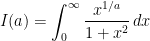
\begin{aligned} I(a)=\int_0^\infty \frac{x^{1/a}}{1+x^2}\,dx \end{aligned}

So this is the integral we’ll be investigating. But in order to see why complex integration will be useful to evaluate real integrals, we’re going to discuss a few ideas and an important theorem that we will need.

First of all, what is complex integration? Well, it can be useful to think of it as line integration in the complex plane. Take a function f:\mathbb{C}\to\mathbb{C} and a C^1 curve \gamma [a,b]\to\mathbb{C}. The integral of f(z) along \gamma is denoted as

\begin{aligned} \int_{\gamma} f(z) dz \end{aligned}

But this doesn’t really help us evaluate it, which we will want to do. Choose a parametrization z\mapsto \gamma(t):\mathbb{R}\to\mathbb{C} be a parametrization of \gamma that is consistent with its direction. Then, the same integral can also be defined as

\begin{aligned} \int_a^b f(\gamma(t)) \,\gamma'(t)dt \end{aligned}

Now this definition will be useful to us. Next, we’ll talk about contours. A contour is a sum of piece-wise continuous whose endpoints are connected so that they all point in one direction. Here are some examples of different contours:

Contours

Now you may be asking yourself how a complex line integral will help us evaluate a real integral that we are after. The main tool that will help us is the Residue Theorem:

Let U be a simply connected open subset, and let f(z) be holomorphic in U\setminus \{a_1,a_2,...,a_k\}. Let \gamma be a closed contour contained in U that encircles all the singularities of f(z). Then, the contour integral of f(z) over \gamma is equal to

\begin{aligned} \int_{\gamma} f(z) dz = 2\pi i\sum_{n=1}^k \text{Res}(f,a_n) \end{aligned}

The residue at a pole, or singularity, depends on the pole’s order. If f(z) has a pole at z=a, then the order of the pole is the smallest integer n, such that \lim_{z\to a} (z-a)^n f(z) is finite. If we know the order of the pole, which ususally isn’t too hard to find, we can calculate the Residue of f at that pole using the following formula:

\begin{aligned} \text{Res}(f,a)=\frac{1}{(n-1)!}\lim_{z \to a} \frac{d^{n-1}}{dz^{n-1}} (z-a)^n f(z) \end{aligned}

In our integral today, we’ll be dealing with a simple pole, where n=1. The formula then reduces to

\begin{aligned} \text{Res}(f,a)=\lim_{z \to a} (z-a) f(z) \end{aligned}

Which is much simpler. We are now ready to tackle our integral! Well almost. We have two more things to go over, and those are branch points and branch cuts. Basically, a branch point of a multi-valued function is a point around which the function is discontinuous on a circle enclosing the point. For the complex natural logarithm, \log z, 0 is a branch point. This is because, starting from the point z=r+0i, and going around the circle counterclockwise, the logarithm gains an argument of 2\pi i. There is thus a discontinuity at the point z=r, as \lim_{\epsilon \to 0^+} \log(r+\epsilon i)=\log r, but \lim_{\epsilon \to 0^-} \log(r+\epsilon i) =\log r + 2\pi i. This stems from the fact that the complex log is a multivalued function.

Finally, branch cuts are the points where the single-valued functions come together to make the multi-valued function. For example, going back to the log function, we can define a branch cut on [0,\infty), letting \text{arg}z \in [0,2\pi i), in such a way that the log function is now single-valued and analytic on \mathbb{C} \setminus [0,\infty).

You may think that this multi-valuedness is just going to cause us problems when evaluating integrals in the complex plane, but it will actually help us with a wide range of integrals, as you will see.

We are now ready to compute the integral we started with, using contour integration. The first step is choosing a contour. When I first started, this step was very mysterious to me and I wasn’t exactly sure which contour to choose. That intuition will come with practice and time as you get to better understand contour integration with different integrands. Today, we’ll be using a special contour named a “keyhole contour”, as you may see why:

Keyhole Contour

Because x^{1/a}=e^{(\log x)/a}, we will have to make a branch cut. In thise case, it will be along the real axis. And we’re going to be choosing \text{arg} z \in [0,2\pi). Basically, we’re going have 4 different integrals, one for each segment of the contour. In this case, we will let f(z)=\frac{ z^{1/a}}{1+z^2}.  I’ll parametrize the large circular part by z=Re^{i\theta} for \theta \in [\epsilon, 2\pi - \epsilon]. The smaller circle will be similarly parameterized. Our contour integral is then
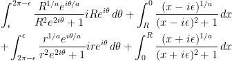
\begin{aligned} \int_{\epsilon}^{2\pi - \epsilon} \frac{ R^{1/a} e^{i\theta/a}}{R^2e^{2i\theta}+1}i Re^{i\theta}\,d\theta + \int_{R}^0  \frac{(x-i\epsilon)^{1/a}}{(x-i\epsilon)^2+1}\,dx \\ + \int_{2\pi-\epsilon}^{\epsilon} \frac{ r^{1/a} e^{i\theta/a}}{r^2e^{2i\theta}+1}i re^{i\theta}\,d\theta + \int_{0}^R  \frac{(x+i\epsilon)^{1/a}}{(x+i\epsilon)^2+1}\,dx \end{aligned}

As wel let R\to\infty and r \to 0, the first and third integrals vanish, leaving us with only the second and fourth. And as we let \epsilon \to 0, our second integral will gain a factor of e^{2\pi i/a}, as the logarithm from the function z^{1/a}=e^{(\log z)/a} has gained an argument of 2\pi i as it circle back to the real axis. Our contour integral is now

\begin{aligned} \left(1-e^{2\pi i/a}\right)\int_0^\infty \frac{x^{1/a}}{x^2+1}\,dx \end{aligned}

Which is very close to our desired integral! Now, you may see the purpose of the keyhole contour. It takes advantage of the fact that the logarithm is multivalued in order to let us compute our integral, as if the log did not gain that argument of 2\pi i, our desired integral would simply vanish from the overall contour integral. We can now use the Residue Theorem to finish the computation. We know that there are two poles at z=\pm i. Summing the Residues and muptiplying them by 2\pi i, we obtain

\begin{aligned} \left(1-e^{2\pi i/a}\right)\int_0^\infty \frac{x^{1/a}}{x^2+1}\,dx=\pi\left(e^{i\pi/2a}+e^{3\pi i/2a}\right) \end{aligned}

After some compuations, we obtain

\begin{aligned} \int_0^\infty \frac{x^{1/a}}{x^2+1}\,dx &= \pi \frac{\sin \left(\frac{\pi}{2a}\right)}{\sin \left(\frac{\pi}{a}\right)} \\ &=\frac{\pi}{2} \sec\left(\frac{\pi}{2a}\right) \end{aligned}

What a beautiful result! This really shows the power of contour integration, and although it can be long to arrive at the result, it is a very useful technique.

Another round of Schwinger parametrization–simpler this time

Hello integral enthusiasts! Today’s we’ll be computing a pretty hard integral using a similar technique to the one used last time. However, we’re going to use the simplified Schwinger parametrization.

Remember that

\begin{aligned} \frac{1}{A(x)^p}=\frac{1}{\Gamma(p)} \int_0^\infty u^{p-1} e^{-u A(x)}\,du \end{aligned}

And choosing p=1, we find that

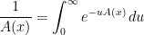
\begin{aligned} \frac{1}{A(x)}= \int_0^\infty e^{-u A(x)}\,du \end{aligned}

We’ll be using this equality for our integral today, which is…

\begin{aligned} I_a^b=\int_{-\infty}^\infty \frac{e^{-ax^2}}{x^2+b^2}\,dx \end{aligned}

This is a pretty daunting integral, as it’s not easy to integrate a combination of inverse polynomials and gaussian functions. But this is where our parametrization comes in! Choosing A(x)=x^2+b^2, we can show that

\begin{aligned} I_a^b&=\int_{-\infty}^\infty \frac{e^{-ax^2}}{x^2+b^2}\,dx \\ &=\int_{-\infty}^\infty e^{-ax^2}\int_0^\infty e^{-u(x^2+b^2)}\,dudx \end{aligned}

And thanks to absolute convergence of our integrals, we can switch the order of integration,

\begin{aligned} I_a^b&= \int_{-\infty}^\infty e^{-ax^2}\int_0^\infty e^{-u(x^2+b^2)}\,dudx \\ &=\int_0^\infty e^{-ub^2}\int_{-\infty}^\infty e^{-x^2(a+u)}\,dxdu \\ &=\sqrt{\pi}\int_0^\infty \frac{e^{-ub^2}}{\sqrt{a+u}}\,du \\ &= \sqrt{\pi}\int_a^\infty \frac{e^{-(\nu-a)b^2}}{\sqrt{\nu}}\,d\nu \\ &= \sqrt{\pi}e^{ab^2} \int_a^\infty \nu^{-1/2} e^{-\nu b^2}\,d\nu \quad \quad \nu=s^2 \\  &=2\sqrt{\pi}e^{ab^2}\int_{\sqrt{a}}^\infty e^{-s^2 b^2}\,ds \end{aligned}

We’ll now substitute s=\lambda/b:

\begin{aligned} I_a^b&= 2\sqrt{\pi}e^{ab^2}\int_{\sqrt{a}}^\infty e^{-s^2 b^2}\,ds \\ &=2\frac{\sqrt{\pi}}{b}e^{a b^2}\int_{b\sqrt{a}}^\infty e^{-\lambda^2}\,d\lambda \end{aligned}

And we can now use the definition of the complementary error function to finish off this integral:

\begin{aligned} \text{erfc}(x)&=1-\text{erf}(x) \\ &= \frac{2}{\sqrt{\pi}} \int_x^\infty e^{-t^2}\,dt \end{aligned}

And using this interesting function, our integral can now be expressed as

\begin{aligned} I_a^b&=2\frac{\sqrt{\pi}}{b}e^{a b^2}\int_{b\sqrt{a}}^\infty e^{-\lambda^2}\,d\lambda \\ &=\frac{\pi}{b} e^{ab^2} \text{erfc}(b\sqrt{a}) \end{aligned}

This means we have the nice result that

\begin{aligned} \int_{-\infty}^\infty \frac{e^{-ax^2}}{x^2+b^2}\,dx=\frac{\pi}{b} e^{ab^2} \text{erfc}(b\sqrt{a}) \end{aligned}

And although the error function is technically not elementary, it is still nice to be able to use it in cases like this one.


Schwinger parametrization

Hello everyone, I’m back today with an article about an integration technique I just recently discovered that’s called Schwinger parametrization. It actually originated in the calculation of loop integrals in Quantum Field Theory.

The method makes use of the following identity, which can be derived by a change of variable in the usual definition of the Gamma function.

\begin{aligned} \frac{1}{\beta^m(x)}=\frac{1}{\Gamma(m)}\int_0^\infty u^{m-1} e^{-u\beta(x)}\,du \end{aligned}

It’s a nice way to deal with integrals involving arbitrary powers of a function in the denominator. In this post and with this technique, I’ll show you that

\begin{aligned} I(n,p)=\int_0^\infty \left(\frac{1}{1+x^n}\right)^p\,dx=\frac{\pi}{\Gamma(p) n}\csc\left(\frac{\pi}{n}\right)\prod_{k=1}^{p-1} \left(p-k-\frac{1}{n}\right) \end{aligned}

Now this can be a pretty hard integral to compute, but Schwinger parametrization allows us to find its value.

First, let’s Schwinger parametrize it, letting \beta(x)=\frac{1}{1+x^n}

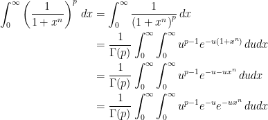
\begin{aligned} \int _0^\infty \left(\frac{1}{1+x^n}\right)^p\,dx &= \int _0^\infty \frac{1}{\left(1+x^n\right)^p}\,dx \\ &= \frac{1}{\Gamma(p)}\int_0^\infty \int_0^\infty u^{p-1} e^{-u(1+x^n)} \,du dx \\ &= \frac{1}{\Gamma(p)}\int_0^\infty \int_0^\infty u^{p-1} e^{-u-ux^n} \,du dx \\ &= \frac{1}{\Gamma(p)}\int_0^\infty \int_0^\infty u^{p-1} e^{-u}e^{-ux^n} \,du dx \end{aligned}

Upon switching the order of integration, we find that

\begin{aligned} \frac{1}{\Gamma(p)}\int_0^\infty \int_0^\infty u^{p-1} e^{-u}e^{-ux^n} \,dx du &= \frac{1}{\Gamma(p)}\int_0^\infty u^{p-1} e^{-u}\,du\int_0^\infty e^{-ux^n} \,dx \\ &= \frac{1}{\Gamma(p)}\int_0^\infty u^{p-1} e^{-u}\,du \int_0^\infty \frac{s^{1/n -1}}{n} e^{-us} \,ds \\ &= \frac{1}{\Gamma(p)}\int_0^\infty u^{p-1} e^{-u}\,du \frac{\Gamma(\frac{1}{n})}{u^{1/n}n} \\ &=\frac{\Gamma\left(1+\frac{1}{n}\right)}{\Gamma(p)}\int_0^\infty u^{p-1/n-1} e^{-u}\,du \end{aligned}

Where we simply used the substitution s=x^n. This last integral can also be expressed in terms of the Gamma function:

\begin{aligned} \frac{\Gamma\left(1+\frac{1}{n}\right)}{\Gamma(p)}\int_0^\infty u^{p-1/n-1} e^{-u}\,du &= \frac{\Gamma\left(1+\frac{1}{n}\right)\Gamma\left(p-\frac{1}{n}\right) }{\Gamma(p)} \end{aligned}

And we have our first result (that will be simplified):

\begin{aligned} \int_0^\infty \frac{1}{\left(1+x^n\right)^p}\,dx=\frac{\Gamma(\frac{1}{n}+1)\Gamma(p-\frac{1}{n})}{\Gamma (p)} \text{ for } pn>1 \end{aligned}

For fixed values of p, we do have nice results:

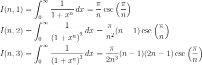
\begin{aligned} I(n,1) &= \int_0^\infty \frac{1}{1+x^n}\,dx=\frac{\pi}{n}\csc\left(\frac{\pi}{n}\right) \\ I(n,2) &= \int_0^\infty \frac{1}{\left(1+x^n\right)^2}\,dx=\frac{\pi}{n^2}(n-1)\csc\left(\frac{\pi}{n}\right) \\ I(n,3) &= \int_0^\infty \frac{1}{\left(1+x^n\right)^3}\,dx=\frac{\pi}{2n^3}(n-1)(2n-1)\csc\left(\frac{\pi}{n}\right) \end{aligned}

This result can be generalized for any integer values of p using some facts about the Gamma function:

\begin{aligned} \frac{\Gamma(\frac{1}{n}+1)\Gamma\left(p-\frac{1}{n}\right)}{\Gamma (p)} &= \frac{\Gamma\left(1+\frac{1}{n})\right)\Gamma\left(1-\frac{1}{n}\right)}{\Gamma(p)}\prod_{k=1}^{p-1} \left(p-k-\frac{1}{n}\right) \end{aligned}

And using the fact that

\begin{aligned} \Gamma\left(1+\frac{1}{n}\right)\Gamma\left(1-\frac{1}{n}\right)= \frac{\pi}{n}\csc\left(\frac{\pi}{n}\right) \end{aligned}

We find

\begin{aligned} \int_0^\infty \left(\frac{1}{1+x^n}\right)^p\,dx=\frac{\pi}{\Gamma(p) n}\csc\left(\frac{\pi}{n}\right)\prod_{k=1}^{p-1} \left(p-k-\frac{1}{n}\right) \end{aligned}

Using this equality, we can even find the L^p norm over [0,\infty) of the function f(x)=\frac{1}{1+x^n}:

\begin{aligned} ||f||_{L^p}&=\left(\int_0^\infty |f|^p\,dx\right)^{1/p} \\ &= \left(\int_0^\infty \left(\frac{1}{1+x^n}\right)^p \,dx\right)^{1/p} \\ &= \sqrt[p]{\frac{\pi}{\Gamma(p) n}\csc\left(\frac{\pi}{n}\right)\prod_{k=1}^{p-1} \left(p-k-\frac{1}{n}\right)} \end{aligned}

The method of brackets in action

In a previous post, I quickly linked a few interesting paper on arXiv about the method of brackets for evaluating integrals. Well I wanted to show you how powerful it can be with a simple but interesting example.

Consider the Mellin transform of

\begin{aligned} f(x)=\sin x \end{aligned}

Or,

\begin{aligned} \mathcal{M}[f](s)=\int_{0}^{\infty}x^{s-1}\sin x\,dx \end{aligned}

Now, some restrictions have to be placed on s to ensure convergence of this integral. First, for our integrand to be integrable around x=0, we need s > -1. Next, we need 1-s > 1, or s<1, to make sure that our integrand goes to zero rapidly enough. Thus, s\in(-1,1).

We also know that the sine function can be expanded into the following nice Taylor series that converges everywhere on \mathbb{R}.

\begin{aligned} \sin x=\sum_{n=0}^{\infty} \frac{(-1)^n}{(2n+1)!} \,x^{2n+1} \end{aligned}

From this paper, we know that we need to map our integral to the following bracket series:

\begin{aligned} \mathcal{M}[f] \mapsto \sum _n \frac{(-1)^n}{(2n+1)!} \langle 2n+s+1 \rangle \end{aligned}

Or, letting \phi_n=\frac{(-1)^n}{\Gamma(n+1)},

\begin{aligned} \mathcal{M}[f] \mapsto \sum _n \phi_n \frac{\Gamma(n+1)}{\Gamma(2n+2)} \langle 2n+s+1 \rangle \end{aligned}

And since, according to Rule 2.2, the a bracket series is given the value of

\begin{aligned} \sum_n \phi_n f(n) \langle an+b \rangle = \frac{1}{|a|} f(n^*) \Gamma(-n^*) \end{aligned}

Where n^* is the solution to the vanishing of the brackets, or equivalently is the solution to the equation an+b=0. In our case, n^*=-(s+1)/2.

Letting s/2=\nu, Our integral is thus equal to

\begin{aligned} \mathcal{M}[f]=\frac{1}{2} \frac{\Gamma(-\nu +\frac{1}{2})}{\Gamma(-2\nu+1)} \, \Gamma\left(\nu+\frac{1}{2}\right) \end{aligned}

And using the Legendre Duplication Formula and the Gamma reflection formula, we can further simplify this mess of Gamma functions into

\begin{aligned} \mathcal{M}(s)=\frac{\pi}{2} \frac{\sec\left(\frac{\pi s}{2}\right)}{\Gamma(1-s)} = \sin\left(\frac{\pi s}{2}\right) \Gamma(s) \end{aligned}

Using the first form, we can easily deduce that value of Dirichlet’s integral by setting s=0 :

\begin{aligned} \mathcal{M}(0)=\int_0^{\infty} \frac{\sin x}{x}\,dx=\frac{\pi}{2} \end{aligned}

And either form allows us to compute a closely related integral:

\begin{aligned} \mathcal{M}(1/2)=\int_0^{\infty} \frac{\sin x}{\sqrt{x}}\,dx=\sqrt{\frac{\pi}{2}} \end{aligned}

So for any s \in (-1,1),

\begin{aligned} \int_0^{+\infty} x^{s-1} \sin x \,dx = \frac{\pi}{2} \frac{\sec\left(\frac{\pi s}{2}\right)}{\Gamma(1-s) } = \sin\left(\frac{\pi s}{2}\right) \Gamma(s) \end{aligned}


Hyperbolic substitutions and Feynman’s

Hey everyone! In this post, we’ll be combining differentiation under the integral sign and hyperbolic subs to evaluate:

\begin{aligned} \int_0^1 \frac{\arctan x}{x\sqrt{1-x^2}}\,dx \end{aligned}

Let’s first try to parameterize the integral, in order to prep it for differentiation:

\begin{aligned} \mathcal{P}(a)=\int_0^1 \frac{\arctan(ax)}{x\sqrt{1-x^2}}\,dx \end{aligned}

After differentiating,

\begin{aligned} \mathcal{P}'(a)&=\int_0^1 \left(\frac{x}{1+a^2x^2}\right)\left(\frac{1}{x\sqrt{1-x^2}}\right)\,dx \\ &= \int_0^1\left(\frac{1}{1+a^2x^2}\right)\left( \frac{1}{\sqrt{1-x^2}}\right)\,dx\end{aligned}

As you can see, the x’s nicely canceled out after differentiating. This parametrization seems to work. But remember that you won’t always find the right parametrization on the first try. Now, let’s try the substitution \displaystyle x=\sin \theta.

\begin{aligned} \mathcal{P}'(a)&=\int_0^{\pi/2}\left(\frac{1}{1+a^2\sin^2\theta}\right)\left( \frac{1}{\sqrt{1-\sin^2\theta}}\right)\cos\theta\, d\theta  \\ &= \int_0^{\pi/2} \frac{d\theta}{1+a^2\sin^2 \theta}\end{aligned}

Notice that by the change of variables \displaystyle \theta\mapsto\frac{\pi}{2}-\theta,

\begin{aligned}\int_0^{\pi/2} \frac{d\theta}{1+a^2\sin^2 \theta}=\int_0^{\pi/2} \frac{d\theta}{1+a^2\cos^2 \theta}  \end{aligned}

We can now substitute \displaystyle \theta\mapsto\arctan t. We can also use the Pythagorean identity \displaystyle 1+\tan^2 \theta=\sec^2\theta, or in our case, \displaystyle \cos^2 =\frac{1}{1+t^2}.

\begin{aligned}\mathcal{P}'(a)&=\int_0^{+\infty} \left(\frac{1}{1+a^2\frac{1}{1+t^2}}\right)\left(\frac{dt}{1+t^2}\right) \\ &=\int_0^{+\infty} \frac{dt}{1+a^2+t^2} \\ &= \frac{1}{\sqrt{1+a^2}}\arctan\left(\frac{t}{\sqrt{1+a^2}}\right)\Biggr|_0^{+\infty} \\ &= \frac{\pi}{2}\frac{1}{\sqrt{1+a^2}}\end{aligned}

We have a nice differential equations that we can solve by separating variables:

\begin{aligned} \mathcal{P}(a)=\frac{\pi}{2}\int \frac{1}{\sqrt{1+a^2}}\,da  \end{aligned}

Here is where the hyperbolic substitution comes in. If you recall that

\displaystyle \cosh^2 \nu -\sinh^2 \nu=1

\displaystyle 1+\sinh^2\nu=\cosh^2\nu

we can substitute \displaystyle a\mapsto \sinh\nu.

\begin{aligned} \mathcal{P}(a)&=\frac{\pi}{2}\int \frac{1}{\sqrt{1+\sinh^2 \nu}}\cosh\nu\,d\nu  \\ &= \frac{\pi}{2} \int \frac{\cosh \nu}{\cosh \nu}\,d\nu \\ &= \frac{\pi}{2}\int d\nu \\ &=\frac{\pi}{2}\nu+C \end{aligned}

What is the constant? Well it’s zero since going back to the original integral, \displaystyle \mathcal{P}(0)=0. And going back to the substitution, \displaystyle \nu=\text{arcsinh }\! a.

\begin{aligned} \mathcal{P}(a)=\frac{\pi}{2} \text{arcsinh }\! a\end{aligned}

And here is our long-awaited result!

\begin{aligned}\int_0^1 \frac{\arctan(ax)}{x\sqrt{1-x^2}}\,dx=\frac{\pi}{2} \text{arcsinh }\! a\end{aligned}

Letting \displaystyle a=1,

\begin{aligned}\int_0^1 \frac{\arctan x}{x\sqrt{1-x^2}}\,dx&=\frac{\pi}{2} \text{arcsinh }\! 1 \\ &=\frac{\pi}{2} \log\left(1+\sqrt{2}\right)\end{aligned}


Convergence of functional sequences

What does it mean for a sequence to converge? What does it mean for a sum to converge? Are there different types of convergence? All these question are fundamental to mathematics, and are usually covered in a Real Analysis class. Even though I–unfortunately–haven’t yet taken that course, I am fascinated by the different mathematical concepts it covers. One of these is the idea of convergence. We’ll focus on the two main types: pointwise convergence and uniform convergence.

Since pointwise convergence is “weaker”, in a sense, than uniform convergence, I think it’s natural to start with it. Here is the formal definition:

Let a sequence of functions (f_n)_{n=1}^{\infty} be defined on an interval I\subseteq\mathbb{R}  where f_n: I\to\mathbb{R} \,\,\,\,\forall n\in\mathbb{N}. The sequence converges pointwise to a function f:I\to\mathbb{R} if

\displaystyle \lim_{n\to\infty} f_n(x)=f(x)

For example, consider the sequence

\displaystyle f_n(x)=x-\frac{1}{n}

It is easy to verify that our sequence converges pointwise to the limit function f(x)=x. Indeed,

\displaystyle \lim_{n\to\infty} \left(x-\frac{1}{n}\right)=x

Now for a little harder example; let the following define a sequence of functions:

\displaystyle f_n(x)=e^{-nx} for x\in[1,5]

Does our sequence converge pointwise on that interval? Let’s check:

\displaystyle \lim_{n\to\infty} e^{-nx}=0 \,\,\,\forall x\in[1,5]

Thus our sequence converges to the limit function f(x)=0 on the interval [1,5]. But what happens if we look at the interval [0,5]? We know that

\displaystyle e^{-nx}\to 0 \,\,\,\forall x\in(0,5] pointwise.

However f_n(0)=1 for all n. This means the limit function is not continuous, despite the fact that every f_n(x) is continuous.

This points to one of the flaws of pointwise convergence: it does not guarantee continuity, and nor does it guarantee differentiability. We need a stronger form of convergence: uniform convergence. But first, there is one definition that we need. Define the supremum norm of f on I as

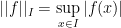
\displaystyle||f||_I=\sup_{x\in I}|f(x)|

We are now ready:

Let a sequence of functions (f_n)_{n=1}^{\infty} be defined on an interval I\subseteq\mathbb{R}  where f_n: I\to\mathbb{R} \,\,\,\,\forall n\in\mathbb{N}. The sequence converges uniformly to a function f(x) if

\displaystyle ||f_n(x)-f(x)||_I\to 0 \,\,\,\,\,\text{as}  \,\,\,\, n\to\infty

Notice that uniform convergence implies pointwise convergence. We can now look at a previous sequence of functions that we know to be pointwise convergent, and check whether it is uniformly convergent. We know that the sequence f_n(x)=e^{-nx} converges pointwise on [1,5]. Checking for uniform convergence:

\displaystyle ||e^{-nx}-0||_{x\in[1,5]}=||e^{-nx}||_{x\in[1,5]}

\displaystyle =e^{-n}\to 0 \,\,\,\,\text{as}\,\,\,\, n\to\infty

Thus the sequence converges uniformly on the interval [1,5]. Let’s now look at a different sequence:

\displaystyle f_n(x)=xe^{-nx}\,\,\,\text{on}\,\,\,[0,\infty)

It is easily verified that the sequence converges pointwise to the limit function f(x)=0. What about uniform convergence?

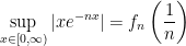
\displaystyle ||xe^{-nx}||_{x\in[0,\infty)}=\sup_{x\in[0,\infty)}|xe^{-nx}|

After differentiating f_n(x) we have that the function attains a maximum at x=\frac{1}{n}.

\displaystyle \sup_{x\in[0,\infty)}|xe^{-nx}|=f_n\left(\frac{1}{n}\right)

\displaystyle =\frac{1}{ne}\to 0\,\,\,\text{as}\,\,\, n\to\infty

Thus our sequence converges uniformly to its limit function f(x)=0 on [0,\infty).

There are many applications of uniform convergence, including the guarantee that the limit function is continuous and differentiable if the sequence function is. These types of convergence can be extended to functional series, with some very interesting results.


A Dirichlet integral

Let’s look at one of the most famous definite integrals,

\displaystyle \int_0^{\infty} \frac{\sin(\omega)}{\omega}\,d\omega

This integral is particularly interesting because it doesn’t yield itself to the standard techniques of integration. What makes it even more interesting are the multitude of ways of evaluating it. Laplace transforms, double integrals and differentiation under the integral sign all work here. I’ll choose to focus on the double integral method; if you wish to learn more about evaluating it using differentiation under the integral sign, you should watch this video, from a friend of mine who does a phenomenal job at explaining it.

Mathematics is not an exact science, like some people tend to think. Especially when talking about integrals. I like to view them as an art, where one needs ample creativity to be proficient in it. And because of this, sometimes there appears to be no logic going from one step to another. This the case here.

To start, first notice that

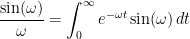
\displaystyle \frac{\sin(\omega)}{\omega}=\int_0^{\infty} e^{-\omega t}\sin(\omega)\,dt

This is what I’m talking about. There is no formula that will lead you to use this fact. Instead, the first person who used this technique was creative enough to come up with this and use it in the evaluation of the integral.

Let’s make a substitution in our original integrand:

\displaystyle \int_0^{\infty} \frac{\sin(\omega)}{\omega}\,d\omega= \int_0^{\infty}\left(\int_0^{\infty} e^{-\omega t}\sin(\omega)\,dt\right) \,d\omega=\int_0^{\infty}\int_0^{\infty} e^{-\omega t}\sin(\omega)\,dt d\omega

We now have a double integral to evaluate. And while you may think this only further complicated the task, it actually helped us. We can now change the order of integration*, a classic move in the evaluation of double integrals.

\displaystyle \int_0^{\infty}\int_0^{\infty} e^{-\omega t}\sin(\omega)\,dt d\omega=\int_0^{\infty}\int_0^{\infty} e^{-\omega t}\sin(\omega)\,d\omega dt

The inner integral can be solved easily by integration by parts, but I prefer a different approach. Note that

\displaystyle Im(e^{i\omega})=\sin(\omega)

Focusing on the inner integral, we can equate these:

\displaystyle \int_0^{\infty} e^{-\omega t}\sin(\omega)\,d\omega=Im\int_0^{\infty} e^{-\omega t}e^{i\omega}\,d\omega=Im\int_0^{\infty} e^{\omega(-t+i)}\,d\omega=\left(Im\frac{e^{\omega(-t+i)}}{-t+i}\right)\Big|_0^{\infty}

To be able to evaluate this, we need to find its imaginary part. After using conjugates and doing some simple arithmetic, we arrive at the result:

\displaystyle Im\left(\frac{e^{\omega(-t+i)}}{-t+1}\right)\Big|_0^{\infty}=\frac{-e^{-\omega t}(t\sin(\omega)+\cos(\omega))}{t^2+1}\Big|_0^{\infty}=\frac{1}{t^2+1}

Remember that this was the inner integral. So we can substitute our new expression back in our original double integral:

\displaystyle \int_0^{\infty}\int_0^{\infty} e^{-\omega t}\sin(\omega)\,d\omega dt=\int_0^{\infty} \frac{1}{t^2+1}\,dt

\displaystyle =\lim_{b\to\infty}\left(\arctan(t)\Big|_0^{b}\right)=\lim_{b\to\infty}\arctan(b)=\boxed{\frac{\pi}{2}}

Thus,

\displaystyle \int_0^{\infty} \frac{\sin(\omega)}{\omega}\,d\omega=\frac{\pi}{2}

Since our function is even, the integral over the whole real line gives

\displaystyle \int_{-\infty}^{\infty} \frac{\sin(\omega)}{\omega}\,d\omega=2\left(\frac{\pi}{2}\right)=\pi

And there’s more! After solving an integral like that, you can make a substitution to get a new result. In this case, if we let

\displaystyle \omega=x^3

\displaystyle d\omega=3x^2\,dx

\displaystyle \int_0^{\infty} \frac{\sin(\omega)}{\omega}\,d\omega=3\int_0^{\infty} \frac{\sin(x^3)}{x}\,dx=\frac{\pi}{2}

This means that

\displaystyle \int_0^{\infty} \frac{\sin(x^3)}{x}\,dx=\frac{\pi}{6}

Doubling the interval of integration,

\displaystyle \int_{-\infty}^{\infty} \frac{\sin(x^3)}{x}\,dx=\frac{\pi}{3}

I think that’s so cool!

We can even generalize for other powers of x. Make the substitution

\displaystyle \omega=x^n

\displaystyle d\omega=nx^{n-1}\,dx

\displaystyle \int_0^{\infty} \frac{\sin(x^n)}{x^n} nx^{n-1}\,dx=n\int_0^{\infty}\frac{\sin(x^n)}{x}\,dx=\frac{\pi}{2}

\displaystyle\int_0^{\infty}\frac{\sin(x^n)}{x}\,dx=\frac{\pi}{2n}

Finally, with this, we can now construct a rather exotic, but beautiful, equality:

\displaystyle \int_0^{\infty}\frac{\sin(\sqrt[\pi]{x^3})}{x}\,dx=\zeta(2)=\frac{\pi^2}{6}


*For a rigorous proof that changing the order of integration is possible, see here.


Leibniz’s rule

Leibniz’s rule is a powerful tool for solving otherwise impossible integrals. Here is one of these:

\displaystyle \int^{\infty}_{-\infty}\frac{\sin(x)}{x}\,dx

Substitution, by parts, partial fractions, try it for yourself, all of these methods will fail to give you an antiderivative. We even had to introduce a special function, named Si(x), just to give it an antiderivative. But our method focuses on solving definite integrals, rather than antiderivatives. “Differentiation under the integral sign”, as we call it, is a direct consequence of Leibniz’s rule, which states

\displaystyle \frac{d}{dt} \left(\int_a^{b}f(x,t)\,dx\right)=\int_a^{b}\frac{\partial}{\partial t} f(x,t)\,dx

The variable t only serves as a parameter, which hopefully helps us integrate when we take its partial derivative. But this rule basically states that–under certain lenient conditions– one may interchange the derivative operator and the integral. But how does that help us with anything?, you ask. Well here is an example: say you want to calculate this definite integral

\displaystyle \int^{1}_{0} \frac{x^2 - 1}{\ln(x)}\,dx

Here again, the usual methods will fail us. And we can’t apply our new rule if we don’t have a parameter t. So let’s introduce a new parameter that, when differentiated, will make it simpler to integrate. Ideally, we would want to get rid of that \ln(x) in the denominator. What if we set t=2 in the exponent of our integrand? Than our whole expression would be a function of t, let’s call it I(t), that we would later evaluate at 2:

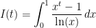
\displaystyle I(t)=\int^{1}_{0} \frac{x^t - 1}{\ln(x)}\,dx

Differentiating with respect to t:

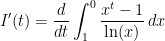
\displaystyle I'(t)=\frac{d}{dt}\int^{0}_{1} \frac{x^t - 1}{\ln(x)}\,dx

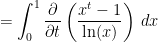
\displaystyle=\int^{1}_{0} \frac{\partial}{\partial t}\left(\frac{x^t - 1}{\ln(x)}\right)\,dx

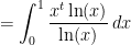
\displaystyle=\int^{1}_{0}\frac{x^t \ln(x)}{\ln(x)}\,dx

\displaystyle=\int^{1}_{0} x^t\,dx

Well this is easier to integrate! The most difficult part is finding the right parameter, and, admittedly, there sometimes won’t be any. But a lot of times, it works nicely just like in our example. We can continue, treating t as a constant in our integration:

\displaystyle I'(t)=\int^{1}_{0} x^t\,dx

\displaystyle=\frac{x^{t+1}}{t+1} \Big|^1_0

\displaystyle= \frac{1}{t+1}

Now, remember, this is the derivative of I(t), not I(t). But that’s not what we want. So to get our original expression, we need to integrate our result with respect to t:

\displaystyle I'(t)=\frac{1}{t+1}

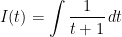
\displaystyle I(t)=\int \frac{1}{t+1}\,dt

\displaystyle I(t)=\ln|t+1|+C

But what is C? Well let’s see if we can find an “initial” condition from our original integrand.

\displaystyle I(t)=\int^{1}_{0} \frac{x^t - 1}{\ln(x)}\,dx

What happens if we set t=0? Then the whole integral equals zero, so I(0)=0:

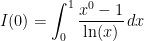
\displaystyle I(0)=\int^{1}_{0} \frac{x^0 - 1}{\ln(x)}\,dx

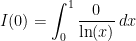
\displaystyle I(0)=\int^{1}_{0} \frac{0}{\ln(x)}\,dx

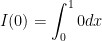
\displaystyle I(0)=\int^{1}_{0} 0 dx

\displaystyle I(0)=0

Knowing these conditions, let’s see what our constant is:

\displaystyle I(0)=\ln|0+1|+C

\displaystyle 0=\ln|1|+C

\displaystyle 0=0+C

\displaystyle C=0

Okay, so we don’t have to worry about the constant since it equals zero. So anyways, we want to evaluate our new expression for I(t) at t=2, because that’s what we substituted t for in the original integrand. We then get:

\displaystyle I(2)=\ln|2+1|

\displaystyle I(2)=\ln|3|

\displaystyle \int^{1}_{0} \frac{x^2 - 1}{\ln(x)}\,dx=\ln(3)

And there is our exact result! Interestingly, we had to solve a more general problem, to then apply it specifically to our problem. What we did allows us to generalize:

\displaystyle \int^{1}_{0} \frac{x^t - 1}{\ln(x)}\,dx=\ln|t+1|

This technique of integration not only allows us to solve some otherwise resisting integrals, but also to generalize to other parameters! Sometimes, we need to actually add a parameter inside the integrand to be able to evaluate it. This technique was actually popularized by Richard Feynman himself, and this is what he said (well wrote) about it in his book Surely, You’re Joking, Mr. Feynman! :

“I had learned to do integrals by various methods shown in a book that my high school physics teacher Mr. Bader had given me. [It] showed how to differentiate parameters under the integral sign – it’s a certain operation. It turns out that’s not taught very much in the universities; they don’t emphasize it. But I caught on how to use that method, and I used that one damn tool again and again. [If] guys at MIT or Princeton had trouble doing a certain integral, [then] I come along and try differentiating under the integral sign, and often it worked. So I got a great reputation for doing integrals, only because my box of tools was different from everybody else’s, and they had tried all their tools on it before giving the problem to me.”

Here’s another integral!

I’m back, and here’s the next entry:

So we’re gonna try to calculate this integral:

\begin{aligned} \int_0^{\infty} \frac{x^a\cos\left(\log x\right)}{1+x^2}\,dx \end{aligned}

Wow, we have a log function inside a cosine?? You could first try transforming this integral into a product of inverse/forwards Laplace transform, but it doesn’t go anywhere (well unless you want to create a whole new function). But you can notice that

\begin{aligned} \cos\left(\log x \right) = \text{Re } \!x^i \end{aligned}

Therefore, our integral can also be expressed as

\begin{aligned} &= \text{Re} \int_0^{\infty} \frac{x^a x^i}{1+x^2}\,dx \\ &= \text{Re} \int_0^{\infty} \frac{x^{a+ i}}{1+x^2}\,dx \end{aligned}

Or

\begin{aligned} \text{Re} \int_0^{\infty} \frac{x^s}{1+x^2}\,dx \end{aligned}

Where we let s=a+i. Now, there are a few different ways we could take to calculate this integral. I’m going to do the trick of converting it into a product of inverse/forwards Laplace transform. We do know that

\begin{aligned} \mathcal{L}\{x^s\}(p)=\frac{\Gamma(s+1)}{p^{s+1}} \end{aligned}

And

\begin{aligned} \mathcal{L}^{-1} \left\{\frac{1}{x^2+1}\right\}(p)=\sin p \end{aligned}

This means that we can transform our original integral into

\begin{aligned} \text{Re } \Gamma(s+1) \int_0^{\infty} \frac{\sin p}{p^{s+1}}\,dp \end{aligned}

This is a pretty hard integral, but we’ve already computed a very similar version of it in a previous post:

\begin{aligned} \int_0^{\infty} p^{s-1} \sin p \,dp = \frac{\pi}{2} \frac{\sec\left(\frac{\pi s}{2}\right)}{\Gamma(1-s)} \end{aligned}

By transforming s\to -s, we can find that

\begin{aligned} \text{Re } \Gamma(s+1) \int_0^{\infty} \frac{\sin p}{p^{s+1}}\,dp &=\text{Re } \Gamma(s+1) \frac{\pi}{2} \frac{\sec\left(\frac{-\pi s}{2}\right)}{\Gamma(1+s)} \\ &= \text{Re } \frac{\pi}{2} \sec\left(\frac{\pi s}{2}\right) \end{aligned}\

By substituting back s=a+i and using the sum formula for cosine, we can see that

\begin{aligned} \text{Re } \frac{\pi}{2} \sec\left(\frac{\pi}{2} (a+i)\right) &= \text{Re } \frac{\pi}{2} \left( \frac{1}{\cos\left(\frac{a\pi}{2}\right)\cos\left(\frac{i\pi }{2}\right) - \sin\left(\frac{a\pi}{2}\right)\sin\left(\frac{i\pi}{2}\right)} \right) \\ \\ &= \text{Re } \frac{\pi}{2} \left( \frac{1}{\cos\left(\frac{a\pi}{2}\right)\cosh\left(\frac{\pi }{2}\right) - i\sin\left(\frac{a\pi}{2}\right)\sinh\left(\frac{\pi}{2}\right)}\right) \\ \\ &= \text{Re } \frac{\pi}{2} \left( \frac{\cos\left(\frac{a\pi}{2}\right)\cosh\left(\frac{\pi }{2}\right) + i\sin\left(\frac{a\pi}{2}\right)\sin\left(\frac{\pi}{2}\right)}{\cos^2\left(\frac{a\pi}{2}\right)\cosh^2\left(\frac{\pi }{2}\right) +\sin^2\left(\frac{a\pi}{2}\right)\sinh^2\left(\frac{\pi}{2}\right)}\right) \\ \\ &=\frac{\pi}{2} \left( \frac{\cos\left(\frac{a\pi}{2}\right)\cosh\left(\frac{\pi }{2}\right) }{\cos^2\left(\frac{a\pi}{2}\right)\cosh^2\left(\frac{\pi }{2}\right) +\sin^2\left(\frac{a\pi}{2}\right)\sinh^2\left(\frac{\pi}{2}\right)} \right) \end{aligned}

We can further simplify this result using half-angle formulas for cosine and sine, as well as for the hyperbolic functions:

\begin{aligned} &=\frac{\pi}{2} \left(\frac{\cos\left(\frac{a\pi}{2}\right)\cosh\left(\frac{\pi }{2}\right) }{\cos^2\left(\frac{a\pi}{2}\right)\cosh^2\left(\frac{\pi }{2}\right) +\sin^2\left(\frac{a\pi}{2}\right)\sinh^2\left(\frac{\pi}{2}\right)} \right) &= \pi\left( \frac{\cos\left(\frac{a\pi}{2}\right)\cosh\left(\frac{\pi }{2}\right)}{\cos(a\pi) +\cosh(\pi)} \right) \end{aligned}

And finally, we obtain the beautiful result:

\begin{aligned} \int_0^{\infty} \frac{x^a\cos\left(\log x\right)}{1+x^2}\,dx = \pi\left( \frac{\cos\left(\frac{a\pi}{2}\right)\cosh\left(\frac{\pi }{2}\right)}{\cos(a\pi) +\cosh(\pi)} \right) \end{aligned}

And here’s a graph of the integrand for different values of a:

desmos-graph (8)


Log hyperbolic tangent integral!

Hello everyone!

In this post, I’ll show you how to evaluate a log hyperb. tangent integral. “What is that?”, you may ask. Well it’s the composition of the log and the hyperbolic tangent function composition all multiplied by another simple natural log:

\begin{aligned} \int_0^{+\infty} \log(x) \log (\tanh x) \,dx \end{aligned}

At first, it may not seem that the convergence is guaranteed, but this integral actually converges absolutely and pretty quickly on [0,+\infty) because the hyperbolic tangent approches 1 very rapidly; this makes the whole integral go to 0 extremely fast. Here is nice graph of the function:graph of log(x)log(tanh(x))

On the other hand, we also have to consider the integrability of the function around x=0. Near 0, we have that

\begin{aligned} \log(x)\log(\tanh x) \sim \log^2(x) \end{aligned}

So if we can show that the integral of whe latter function is integrable around x=0, then we know that our integral is also integrable. If we consider its integral on [0,1], We have that

 \begin{aligned} \int_0^1 \log^2 x\,dx=\int_{0}^{+\infty}  x^2 e^{-x}\,dx= 2<+\infty \end{aligned}

This means that our integrand is integrable around 0, and we can safely go one to actually calculate its value.

To evaluate this challenging integral, we will use differentiation under the integral sign on the following integral:

 \begin{aligned} I(b)=\int_0^{+\infty} x^b \log(\tanh x)\,dx \end{aligned}

Our goal is then to find I'(0):

\begin{aligned} I'(0)=\int_0^{+\infty} \log(x)\log(\tanh x)\,dx \end{aligned}

By expanding the hyperbolic tangent into is exponentials,

\begin{aligned} I(b)&=\int_0^{+\infty} x^b \left(\log(1-e^{-2x})-\log(1+e^{-2x})\right)\,dx \\ &= \int_0^{+\infty} x^b \log(1-e^{-2x})\,dx-\int_0^{+\infty} x^b\log(1+e^{-2x})\,dx \end{aligned}

And after using the Maclaurin expansion of the natural log, we have that

\begin{aligned} I(b)&=-\int_0^{+\infty} x^b \sum_{n=1}^{+\infty} \frac{e^{-2nx}}{n}\,dx-\int_0^{+\infty} x^b \sum_{n=1}^{+\infty} (-1)^{n+1}\frac{e^{-2nx}}{n}\,dx \\ \\ &= -\sum_{n=1}^{+\infty} \int_0^{+\infty}  \frac{x^be^{-2nx}}{n}\,dx-\sum_{n=1}^{+\infty} \int_0^{+\infty} (-1)^{n+1}\frac{ x^b e^{-2nx}}{n}\,dx \\ \\ &= -\frac{\Gamma(b+1)}{2^{b+1}} \sum_{n=1}^{+\infty} \frac{1}{n^{b+2}} - \frac{\Gamma(b+1)}{2^{b+1}} \sum_{n=1}^{+\infty} \frac{(-1)^{n+1}}{n^{b+2}} \end{aligned}

Where we have used the fact that

\begin{aligned} \int_0^{+\infty} x^b e^{-sx}\,dx=\frac{\Gamma(b+1)}{s^{b+1}} \end{aligned}

We can use the series definition of the Riemann zeta function as well as the Dirichlet eta function to further simplify this expression:

\begin{aligned} I(b)&=-\frac{\Gamma(b+1)}{2^{b+1}} \zeta(b+2)-\frac{\Gamma(b+1)}{2^{b+1}} \eta(b+2) \end{aligned}

And after using this relationship between the zeta and eta function,

\begin{aligned} \eta(s)=\zeta(s)\left(1-2^{1-s}\right) \end{aligned}

Our expression becomes

\begin{aligned} I(b)&=-\frac{\Gamma(b+1)}{2^{b+1}} \zeta(b+2)-\frac{\Gamma(b+1)}{2^{b+1}} \zeta(b+2)\left(1-2^{-(b+1)}\right) \\ \\ &=-\frac{\Gamma(b+1)\zeta(b+2)}{2^{b+1}} \left(2-2^{-(b+1)}\right) \\ \\ &= -\frac{\Gamma(b+1)\zeta(b+2)}{2^b}  \left(1-2^{-(b+2)}\right) \end{aligned}

And upon differentiating, we find that

\begin{aligned} I'(b)&=\frac{-\Gamma(b+1)\left[\psi^{(0)}(b+1)\zeta(b+2)+\zeta'(b+2)\right] + \Gamma(b+1_\zeta(b+2)\log 2}{2^b} \left(1-2^{-(b+2)}\right) - \frac{\Gamma(b+1)\zeta(b+2)\log 2}{2} \end{aligned}

And upon setting b=0, we find that

\begin{aligned} I'(0)&=-\frac{3}{4}\left(\psi^{(0)}(1)\zeta(2)+\zeta'(2)\right) + \frac{\zeta(2)\log 2}{2} \end{aligned}

And we have finally found the value of our integral!:

\begin{aligned} \int_0^{+\infty} \log x\log(\tanh x)\,dx&=-\frac{3}{4}\left(\psi^{(0)}(1)\zeta(2)+\zeta'(2)\right) + \frac{\zeta(2)\log 2}{2} \end{aligned}