Hello everyone, and welcome to this exciting post! Today, I’ll be showing you how to use contour integration, a very useful technique from complex analysis, to evaluate a certain integral. What’s nice about contour integration is that it allows you to evaluate so many integrals that you could not otherwise, as a lot of integrands have no elementary anti-derivative. Now, the integral we’ll be focusing on today can be computed using real methods, but I wanted to start using contour integration on this blog. And we won’t even be starting with an “easy” example, as this integral will make us discuss branch points, branch cuts and other things like that from complex analysis. But that will only make it more interesting!
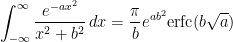
So this is the integral we’ll be investigating. But in order to see why complex integration will be useful to evaluate real integrals, we’re going to discuss a few ideas and an important theorem that we will need.
First of all, what is complex integration? Well, it can be useful to think of it as line integration in the complex plane. Take a function 

![\gamma [a,b]\to\mathbb{C}](https://s0.wp.com/latex.php?latex=%5Cgamma+%5Ba%2Cb%5D%5Cto%5Cmathbb%7BC%7D&bg=ffffff&fg=333333&s=0&c=20201002)


But this doesn’t really help us evaluate it, which we will want to do. Choose a parametrization 

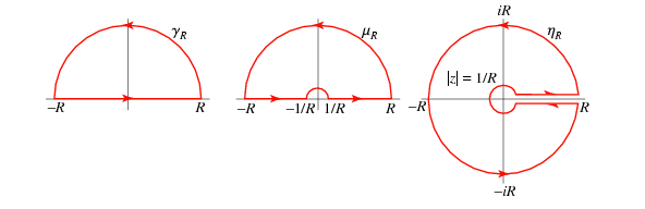
Now this definition will be useful to us. Next, we’ll talk about contours. A contour is a sum of piece-wise continuous whose endpoints are connected so that they all point in one direction. Here are some examples of different contours:
Now you may be asking yourself how a complex line integral will help us evaluate a real integral that we are after. The main tool that will help us is the Residue Theorem:
Let 

The residue at a pole, or singularity, depends on the pole’s order. If 


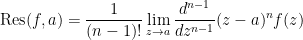
In our integral today, we’ll be dealing with a simple pole, where 

Which is much simpler. We are now ready to tackle our integral! Well almost. We have two more things to go over, and those are branch points and branch cuts. Basically, a branch point of a multi-valued function is a point around which the function is discontinuous on a circle enclosing the point. For the complex natural logarithm, 


Finally, branch cuts are the points where the single-valued functions come together to make the multi-valued function. For example, going back to the log function, we can define a branch cut on 


You may think that this multi-valuedness is just going to cause us problems when evaluating integrals in the complex plane, but it will actually help us with a wide range of integrals, as you will see.
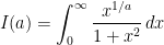
We are now ready to compute the integral we started with, using contour integration. The first step is choosing a contour. When I first started, this step was very mysterious to me and I wasn’t exactly sure which contour to choose. That intuition will come with practice and time as you get to better understand contour integration with different integrands. Today, we’ll be using a special contour named a “keyhole contour”, as you may see why:

Because 


![\theta \in [\epsilon, 2\pi - \epsilon]](https://s0.wp.com/latex.php?latex=%5Ctheta+%5Cin+%5B%5Cepsilon%2C+2%5Cpi+-+%5Cepsilon%5D&bg=ffffff&fg=333333&s=0&c=20201002)
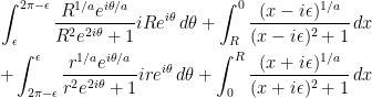
As wel let 


Which is very close to our desired integral! Now, you may see the purpose of the keyhole contour. It takes advantage of the fact that the logarithm is multivalued in order to let us compute our integral, as if the log did not gain that argument of 
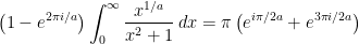
After some compuations, we obtain

What a beautiful result! This really shows the power of contour integration, and although it can be long to arrive at the result, it is a very useful technique.
 , we find that
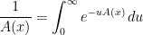

 , we can show that

 :
: