A Dirichlet integral

Posted on September 4, 2017 by philosophicalmath

Let’s look at one of the most famous definite integrals,

$\displaystyle \int_0^{\infty} \frac{\sin(\omega)}{\omega}\,d\omega$

This integral is particularly interesting because it doesn’t yield itself to the standard techniques of integration. What makes it even more interesting are the multitude of ways of evaluating it. Laplace transforms, double integrals and differentiation under the integral sign all work here. I’ll choose to focus on the double integral method; if you wish to learn more about evaluating it using differentiation under the integral sign, you should watch this video, from a friend of mine who does a phenomenal job at explaining it.

Mathematics is not an exact science, like some people tend to think. Especially when talking about integrals. I like to view them as an art, where one needs ample creativity to be proficient in it. And because of this, sometimes there appears to be no logic going from one step to another. This the case here.

To start, first notice that

$\displaystyle \frac{\sin(\omega)}{\omega}=\int_0^{\infty} e^{-\omega t}\sin(\omega)\,dt$

This is what I’m talking about. There is no formula that will lead you to use this fact. Instead, the first person who used this technique was creative enough to come up with this and use it in the evaluation of the integral.

Let’s make a substitution in our original integrand:

$\displaystyle \int_0^{\infty} \frac{\sin(\omega)}{\omega}\,d\omega= \int_0^{\infty}\left(\int_0^{\infty} e^{-\omega t}\sin(\omega)\,dt\right) \,d\omega=\int_0^{\infty}\int_0^{\infty} e^{-\omega t}\sin(\omega)\,dt d\omega$

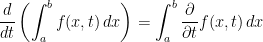
We now have a double integral to evaluate. And while you may think this only further complicated the task, it actually helped us. We can now change the order of integration*, a classic move in the evaluation of double integrals.

$\displaystyle \int_0^{\infty}\int_0^{\infty} e^{-\omega t}\sin(\omega)\,dt d\omega=\int_0^{\infty}\int_0^{\infty} e^{-\omega t}\sin(\omega)\,d\omega dt$

The inner integral can be solved easily by integration by parts, but I prefer a different approach. Note that

$\displaystyle Im(e^{i\omega})=\sin(\omega)$

Focusing on the inner integral, we can equate these:

$\displaystyle \int_0^{\infty} e^{-\omega t}\sin(\omega)\,d\omega=Im\int_0^{\infty} e^{-\omega t}e^{i\omega}\,d\omega=Im\int_0^{\infty} e^{\omega(-t+i)}\,d\omega=\left(Im\frac{e^{\omega(-t+i)}}{-t+i}\right)\Big|_0^{\infty}$

To be able to evaluate this, we need to find its imaginary part. After using conjugates and doing some simple arithmetic, we arrive at the result:

$\displaystyle Im\left(\frac{e^{\omega(-t+i)}}{-t+1}\right)\Big|_0^{\infty}=\frac{-e^{-\omega t}(t\sin(\omega)+\cos(\omega))}{t^2+1}\Big|_0^{\infty}=\frac{1}{t^2+1}$

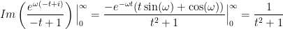
Remember that this was the inner integral. So we can substitute our new expression back in our original double integral:

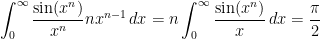
$\displaystyle \int_0^{\infty}\int_0^{\infty} e^{-\omega t}\sin(\omega)\,d\omega dt=\int_0^{\infty} \frac{1}{t^2+1}\,dt$

$\displaystyle =\lim_{b\to\infty}\left(\arctan(t)\Big|_0^{b}\right)=\lim_{b\to\infty}\arctan(b)=\boxed{\frac{\pi}{2}}$

Thus,

$\displaystyle \int_0^{\infty} \frac{\sin(\omega)}{\omega}\,d\omega=\frac{\pi}{2}$

Since our function is even, the integral over the whole real line gives

$\displaystyle \int_{-\infty}^{\infty} \frac{\sin(\omega)}{\omega}\,d\omega=2\left(\frac{\pi}{2}\right)=\pi$

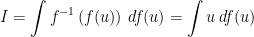
And there’s more! After solving an integral like that, you can make a substitution to get a new result. In this case, if we let

$\displaystyle \omega=x^3$

$\displaystyle d\omega=3x^2\,dx$

$\displaystyle \int_0^{\infty} \frac{\sin(\omega)}{\omega}\,d\omega=3\int_0^{\infty} \frac{\sin(x^3)}{x}\,dx=\frac{\pi}{2}$

This means that

$\displaystyle \int_0^{\infty} \frac{\sin(x^3)}{x}\,dx=\frac{\pi}{6}$

Doubling the interval of integration,

$\displaystyle \int_{-\infty}^{\infty} \frac{\sin(x^3)}{x}\,dx=\frac{\pi}{3}$

I think that’s so cool!

We can even generalize for other powers of x. Make the substitution

$\displaystyle \omega=x^n$

$\displaystyle d\omega=nx^{n-1}\,dx$

$\displaystyle \int_0^{\infty} \frac{\sin(x^n)}{x^n} nx^{n-1}\,dx=n\int_0^{\infty}\frac{\sin(x^n)}{x}\,dx=\frac{\pi}{2}$

$\displaystyle\int_0^{\infty}\frac{\sin(x^n)}{x}\,dx=\frac{\pi}{2n}$

Finally, with this, we can now construct a rather exotic, but beautiful, equality:

$\displaystyle \int_0^{\infty}\frac{\sin(\sqrt[\pi]{x^3})}{x}\,dx=\zeta(2)=\frac{\pi^2}{6}$

*For a rigorous proof that changing the order of integration is possible, see here.

Inverse Integration Technique

Posted on August 15, 2017 by philosophicalmath

A lot of times, integral of inverse functions can be very hard to compute. However, there exists this great “theorem” that allows you to easily find the antiderivative of the inverse of a function, if you know that integral of the function itself. So here it is:

$\displaystyle \int f^{-1}(x)\,dx=x\,f^{-1}(x)-\left(F\circ f^{-1}\right)(x)+C$

Where $F$ denotes the primitive of our function $f(x)$ . The proof is actually pretty easy, so let’s do it now. It relies on a simple substitution and one iteration of integration by parts.

$\displaystyle I=\int f^{-1}(x)\,dx$

Now, we let $x=f(u)$ .

$\displaystyle I=\int f^{-1}\left(f(u)\right)\,df(u)=\int u\,df(u)$

We can now integrate by parts:

$\displaystyle I=\int u\,df(u)=u\,f(u) - \int f(u)\,du= u\,f(u) - F(u) + C$

And all we have left to do is to substitute back in our original variable:

$\displaystyle I=u\,f(u) - F(u) + C=x\,f^{-1}(x)\, -\left(F \circ f^{-1}\right)(x) + C$

And that’s the proof! Short but so useful. Alright, let’s put it to the test by trying to find the primitive of $\tan^{-1}(x)$ . From our formula,

$\displaystyle \int \tan^{-1}(x)\,dx=x\,\tan^{-1}(x)-\left(F\circ f^{-1}\right)(x)+C$

So all we need to do is find the integral of $\tan(x)$ , pretty easy:

$\displaystyle \int \tan(x)\,dx=\int \frac{\sin(x)}{\cos(x)}\,dx=-\int\frac{du}{u}=-\ln|u|=\ln|\sec(x)|$

Substituting this result in our formula,

$\displaystyle \int \tan^{-1}(x)\,dx=x\,\tan^{-1}(x)-\ln|\sec(\tan^{-1}(x))|+C$

But ideally, we would like to simplify that mess inside the natural log. How do we do that? Back to basics: construct a right triangle who has an acute angle of $\theta=\tan^{-1}(x)$ . We are then looking for $\sec(\theta)$ . After using our dear Pythagoras’ theorem, we end up with the following results:

$\displaystyle \sec(\tan^{-1}(x))=\sec(\theta)=\sqrt{x^2+1}$

Still a little messy, but not as bad as our previous expression, right? We then end up with

$\displaystyle \int \tan^{-1}(x)\,dx=x\,\tan^{-1}(x)-\ln|\sqrt{x^2+1}|+C$

$\displaystyle \int \tan^{-1}(x)\,dx=x\,\tan^{-1}(x)-\frac{1}{2}\ln|x^2+1|+C$

And technically, we don’t need the absolute value bars because the expression inside is bound to be positive, but don’t they look cooler?

Leibniz’s rule

Posted on July 22, 2017 by philosophicalmath

Leibniz’s rule is a powerful tool for solving otherwise impossible integrals. Here is one of these:

$\displaystyle \int^{\infty}_{-\infty}\frac{\sin(x)}{x}\,dx$

Substitution, by parts, partial fractions, try it for yourself, all of these methods will fail to give you an antiderivative. We even had to introduce a special function, named Si(x), just to give it an antiderivative. But our method focuses on solving definite integrals, rather than antiderivatives. “Differentiation under the integral sign”, as we call it, is a direct consequence of Leibniz’s rule, which states

$\displaystyle \frac{d}{dt} \left(\int_a^{b}f(x,t)\,dx\right)=\int_a^{b}\frac{\partial}{\partial t} f(x,t)\,dx$

The variable t only serves as a parameter, which hopefully helps us integrate when we take its partial derivative. But this rule basically states that–under certain lenient conditions– one may interchange the derivative operator and the integral. But how does that help us with anything?, you ask. Well here is an example: say you want to calculate this definite integral

$\displaystyle \int^{1}_{0} \frac{x^2 - 1}{\ln(x)}\,dx$

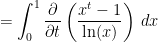
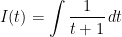
Here again, the usual methods will fail us. And we can’t apply our new rule if we don’t have a parameter t. So let’s introduce a new parameter that, when differentiated, will make it simpler to integrate. Ideally, we would want to get rid of that $\ln(x)$ in the denominator. What if we set $t=2$ in the exponent of our integrand? 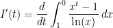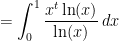Than our whole expression would be a function of t, let’s call it $I(t)$ , that we would later evaluate at 2:

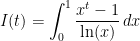
$\displaystyle I(t)=\int^{1}_{0} \frac{x^t - 1}{\ln(x)}\,dx$

Differentiating with respect to t:

$\displaystyle I'(t)=\frac{d}{dt}\int^{0}_{1} \frac{x^t - 1}{\ln(x)}\,dx$

$\displaystyle=\int^{1}_{0} \frac{\partial}{\partial t}\left(\frac{x^t - 1}{\ln(x)}\right)\,dx$

$\displaystyle=\int^{1}_{0}\frac{x^t \ln(x)}{\ln(x)}\,dx$

$\displaystyle=\int^{1}_{0} x^t\,dx$

Well this is easier to integrate! The most difficult part is finding the right parameter, and, admittedly, there sometimes won’t be any. But a lot of times, it works nicely just like in our example. We can continue, treating t as a constant in our integration:

$\displaystyle I'(t)=\int^{1}_{0} x^t\,dx$

$\displaystyle=\frac{x^{t+1}}{t+1} \Big|^1_0$

$\displaystyle= \frac{1}{t+1}$

Now, remember, this is the derivative of $I(t)$ , not $I(t)$ . But that’s not what we want. So to get our original expression, we need to integrate our result with respect to t:

$\displaystyle I'(t)=\frac{1}{t+1}$

$\displaystyle I(t)=\int \frac{1}{t+1}\,dt$

$\displaystyle I(t)=\ln|t+1|+C$

But what is C? Well let’s see if we can find an “initial” condition from our original integrand.

$\displaystyle I(t)=\int^{1}_{0} \frac{x^t - 1}{\ln(x)}\,dx$

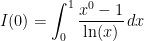
What happens if we set $t=0$ ? Then the whole integral equals zero, so $I(0)=0$ :

$\displaystyle I(0)=\int^{1}_{0} \frac{x^0 - 1}{\ln(x)}\,dx$

$\displaystyle I(0)=\int^{1}_{0} \frac{0}{\ln(x)}\,dx$

$\displaystyle I(0)=\int^{1}_{0} 0 dx$

$\displaystyle I(0)=0$

Knowing these conditions, let’s see what our constant is:

$\displaystyle I(0)=\ln|0+1|+C$

$\displaystyle 0=\ln|1|+C$

$\displaystyle 0=0+C$

$\displaystyle C=0$

Okay, so we don’t have to worry about the constant since it equals zero. So anyways, we want to evaluate our new expression for $I(t)$ at $t=2$ , because that’s what we substituted t for in the original integrand. We then get:

$\displaystyle I(2)=\ln|2+1|$

$\displaystyle I(2)=\ln|3|$

$\displaystyle \int^{1}_{0} \frac{x^2 - 1}{\ln(x)}\,dx=\ln(3)$

And there is our exact result! Interestingly, we had to solve a more general problem, to then apply it specifically to our problem. What we did allows us to generalize:

$\displaystyle \int^{1}_{0} \frac{x^t - 1}{\ln(x)}\,dx=\ln|t+1|$

This technique of integration not only allows us to solve some otherwise resisting integrals, but also to generalize to other parameters! Sometimes, we need to actually add a parameter inside the integrand to be able to evaluate it. This technique was actually popularized by Richard Feynman himself, and this is what he said (well wrote) about it in his book Surely, You’re Joking, Mr. Feynman! :

“I had learned to do integrals by various methods shown in a book that my high school physics teacher Mr. Bader had given me. [It] showed how to differentiate parameters under the integral sign – it’s a certain operation. It turns out that’s not taught very much in the universities; they don’t emphasize it. But I caught on how to use that method, and I used that one damn tool again and again. [If] guys at MIT or Princeton had trouble doing a certain integral, [then] I come along and try differentiating under the integral sign, and often it worked. So I got a great reputation for doing integrals, only because my box of tools was different from everybody else’s, and they had tried all their tools on it before giving the problem to me.”

Gabriel’s Horn

Posted on July 2, 2017 by philosophicalmath

The Math

In this post, we’ll take a look at Gabriel’s Horn, an intriguing mathematical paradox. “Gabriel’s Horn” is the function $f(x)=\frac{1}{x}$ revolved around the positive x-axis. This will create a solid of revolution that looks something like this:

Gabriel Trompette

As you can see, as x approaches infinity, the volume and surface area should tend to zero. Or it seems so… Not so fast! Lets do the math:

For convenience, we will find both the surface area of the solid and the volume from x=1. We cannot start at x=0 since the function $\frac{1}{x}$ is not defined at that point.

To calculate the volume enclosed in a solid of revolution that is created by revolving the curve $f(x)$ from $x_1$ to $x_2$ , we use this formula:

$\displaystyle \pi\int^{x_2}_{x_1} f(x)^2\,dx$

Intuitively, it makes sense: it is multiplying the area of a disk of radius $f(x)$ by $dx$ and then integrating over an interval to calculate the volume. However, the rigorous derivation takes longer, and probably needs a whole post to itself. We will now check if the volume of the “Horn” converges as x goes to infinity. Remember that in our case, $f(x)= \frac{1}{x}$

$\displaystyle \pi\int^{\infty}_{1}\left(\frac{1}{x}\right)^2\,dx$

= $\displaystyle \lim_{b\to\infty} \pi \left(\frac{-1}{x}\right) \Big|_1^b$

= $\displaystyle \lim_{b\to\infty} \pi \left(\frac{-1}{b} - \left(\frac{-1}{1}\right)\right)$

= $\displaystyle \pi \left(0+1\right)$

= $\pi$

The volume does indeed converge as x approaches infinity, specifically to $\pi$ units cubed. Now that we have shown that Gabriel’s Horn has a definite volume when x tends to infinity, lets see what happens to its surface area. To calculate the surface area of a function $f(x)$ revolved around the x-axis, we need to use something else: something that factors in the Pythagorean Theorem:

$\displaystyle 2\pi\int^{x_2}_{x_1} f(x) \sqrt{1+\left(\frac{df}{dx}\right)^2}\,dx$

$\displaystyle =2\pi\int^{\infty}_{1} \frac{1}{x} \sqrt{1+\left(\frac{1}{x^4}\right)}\,dx$

These integrals can be especially tricky to evaluate because of the square root. More often than not, you will have to use some trigonometric substitution–if the integrand even has a closed-form antiderivative… However, we do not have to directly evaluate our integrand: we can use the comparison test. This test says that if

$\displaystyle 0\le f(x)\le g(x)\,\,\forall \,x \in [a,\infty)$ and

$\displaystyle \int^{\infty}_a f(x)\,dx$ diverges, then

$\displaystyle \int^{\infty}_a g(x)\,dx$ will also diverge.

Using this test, we can check if our integral diverges without having to actually compute the antiderivative. We know that

$\displaystyle \int^{\infty}_1 \frac{1}{x}\,dx$ diverges and we also know that

$\displaystyle \frac{1}{x} \le\frac{1}{x} \sqrt{1+\left(\frac{1}{x^4}\right)}\,\, \forall\,x \in [1,\infty)$ Since

$\displaystyle 1\le\sqrt{1+\left(\frac{1}{x^4}\right)}\,\, \forall\,x\in\mathbb{R}$

Hence we can use the comparison test to deduce the convergence or divergence of our integral:

$\displaystyle \int^{\infty}_1 \frac{1}{x}\,dx$

= $\displaystyle \lim_{b\to\infty} \ln \Big|_1^b$

= $\displaystyle \lim_{b\to\infty} \ln(b) - \ln(1)$

= $\displaystyle \,\,\infty$

We have now proved the divergence of $\frac{1}{x}$ on the interval $[1,\infty)$ . Since

$\displaystyle \frac{1}{x} \le\frac{1}{x} \sqrt{1+\left(\frac{1}{x^4}\right)}\,\, \forall\,x \in [1,\infty)$

$\displaystyle \int^{\infty}_{1} \frac{1}{x} \sqrt{1+\left(\frac{1}{x^4}\right)}\,dx$ will also diverge.

The Paradox

Here is the paradox: how can something have infinite surface area but finite volume? Some people also call it the Painter’s Paradox: how could a solid be filled with a finite amount of paint, yet require an infinite amount of paint to covers its surface?

However, mathematically, this is not as much as a paradox as it may seem. Theoretically, a finite amount of paint could cover infinite area, if the thickness of the coat becomes infinitely small, small enough to compensate for the ever-increasing area. In the physical world, there will be a point where not even an atom will fit anymore in the Horn after we fill it with 3.1419… liters of paint. As for surface area, the same can be said. There will a point where the radius of the solid is so small that not even the smallest particle of paint will fit on there. Here, we can see the difference between the continuous mathematical world and the discrete physical world, something that becomes increasingly important when dealing with infinite mathematical models.

It is also interesting to note that it is impossible to have infinite volume and finite area, that is the converse is not true. Careful mathematical reasoning is necessary in these kinds of situation. Relying on human logic alone can often lead us astray and make us susceptible to logical fallacies.

Mathematical Poetry

Mathematical musings and updates

Tag Archives: Calculus